Splines in Onshape

Introduction

Recently I’ve been experimenting with Onshape in the context of a couple of different projects, from designing parts for a microscope to designing jewellery. As a Linux user, I often find myself struggling with the limited capabilities of native CAD tools on Linux, so the ability to do CAD work in a browser on any platform is fantastic. And Onshape is not just a toy: it has some truly impressive capabilities that can compete with high-end desktop-based CAD systems, and it gets better every few weeks, with a release pace that is unparalleled in any other tool that I’m familiar with. (N.B. I have no association with the company, I’m just a happy user.)

One feature that I look for in any CAD system is a programming language or extension API. Most CAD tasks have some degree of structure, and I like the idea of writing code to simplify repetitive tasks. For example, when designing jewellery, one frequently needs to design settings for jewels, and it would be a painstaking process to build these each time from scratch. Onshape’s FeatureScript language is brilliant for this: once I’ve written my custom ‘features’ in FeatureScript, they behave as first-class citizens in the Onshape GUI, and I can simply insert a ‘setting’ or ‘prong’ with a given set of parameters.

If you’ve done any programming before, FeatureScript is quite simple to get started with. The syntax is quite similar to other procedural languages so it takes only a few days before it becomes second nature. One of the aspects that I’ve struggled with, though, it the documentation, which doesn’t always tell you everything you want or need to know. To be fair there is a wealth of FeatureScript examples you can refer to, both from the Onshape team and from users, but it’s not always clear where to start.

For my designs I needed to draw a lot of curves (and then to offset those curves), and while I could do approximately what I wanted in the GUI, it took me a long time to figure out how to do it in FeatureScript as part of my custom features. This article is an attempt to explain some of the missing links for those following in my footsteps. I’ll start with some basic background on splines, then proceed to describe how to draw 2D splines (in a sketch), how to draw 3D splines and how to offset curves. This article is a condensed version of longer pair of posts on my blog; if you’re craving more mathematics, you can refer to that version.

Basics of splines

There’s a lot of mathematical jargon around splines and polynomials; I’ll try to use both the technically correct terms and plain English where possible.

A spline is a piecewise polynomial. The curve is made up of one or more pieces, where each piece is a polynomial. The polynomials are normally chosen such that they “match up” at the transitions and you end up with something that looks like a single continuous curve. There can be various definitions of “matching up”, however to produce a visually smooth curve, at least the function values and the first derivative need to match (C1 continuity), and usually the second derivative is also chosen to match (C2 continuity).

In the case of Onshape splines used in sketches, the pieces are normally cubic polynomials — polynomials of maximum degree 3 — in two dimensions x and y. However, I should be clearer what I mean by that, as there could be at least three different things that could be meant by cubic polynomials in two dimensions:

Explicit form: y=f(x):
y = ax³ + bx² + cx + d
(defined uniquely by 4 free constants: a,b,c,d)

Parametric form: x=f(t), y=g(t) for some parameter t:
x = at³ + bt² + ct + d
y = et³ + ft² + gt + h
(defined uniquely by 8 free constants: a,b,c,d,e,f,g,h)

Implicit form: f(x,y)=0:
ax³ + bx²y + cxy² + dy³ + ex² + fxy + gy² + hx + ky + l = 0
(defined uniquely by 10 free constants: a,b,c,d,e,f,g,h,k,l)

The explicit form can produce, say, a parabola y=x², but can’t produce a parabola rotated by 90 degrees. Therefore it makes little sense for software such as Onshape which must be able to produce curves in any orientation.

The implicit form is the most powerful, in that it can express curves that can’t be expressed in the other two forms, but it is difficult to evaluate the set of points that are part of the curve.

Therefore, as might be expected, Onshape curves are of the parametric type: a curve in two dimensions is produced parametrically by evaluating functions x(t) and y(t) for t from 0 to 1. The functions x(t) and y(t) are splines: there may, for example, be one polynomial piece from t=0 to t=0.5 and one from t=0.5 to t=1. Some of the FeatureScript functions related to curves, such as evEdgeTangentLine() and evEdgeCurvature(), take this parameter t as an argument.

Drawing 2D splines – single polynomial piece

Splines can be created programmatically in an Onshape sketch using the skFitSpline() function. First let’s start with a curve with only one polynomial piece between two points (0,0) and (100,100). In FeatureScript we can write:

skFitSpline(sketch, "spline1", {
        "points" : [
            vector(0,0) * meter,
            vector(100,100) * meter
        ],
        "startDerivative" : vector(150,0) * meter,
        "endDerivative" : vector(0,150) * meter
});

Here is the result:

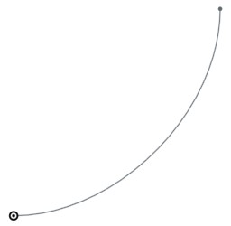
Note that I’ve specified a startDerivative and endDerivative that specify the starting and ending direction; if I had only specified a start and end point then the result would have just been a straight line.

When I was first experimenting with this, my first question was: why do the start and end derivatives have length units (in this case, 150 meters)? With a bit of experimentation it’s clear that these these vectors should be scaled together with the curve, i.e. if we scale the curve up by a factor of two we should also double the startDerivative and endDerivative. Also, a larger magnitude makes the curve launch with more momentum in the given direction; for example, here is the curve with startDerivative increased to (500 meters,0):

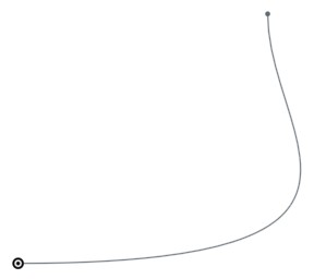
But what does the magnitude of these vectors actually mean?

It all becomes clearer, however, when you consider the curves in parametric form as described in the previous section: x=f(t) and y=f(t). It turns out that the given derivative vectors are the derivatives of (x(t), y(t)) with respect to the parameter t (i.e. (dx/dt, dy/dt)) at t=0 and t=1. If this is too abstract to visualize, there is also a simple mapping to Bézier control points that I’ll explain below.

It turns out that the start point and end point, and the two derivative vectors – four (x,y) pairs in total – uniquely define the eight parameters of the parametric cubic polynomial. Thus, any parametric cubic polynomial can be specified in this way.

Drawing Bézier curves

If you are familiar with Bézier curves the above discussion will sound familiar. A Bézier curve is defined by four control points (call them P₁, P₂, P₃, P₄). The curve launches from P₁ in the direction of P₂, and then approaches P₄ from the direction of P₃. If P₂ is further away from P₁, then the curve launches with more momentum in the given direction.

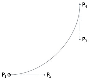
It turns out that these formulations are equivalent with a tiny amount of maths, and if you have the Bézier control points, you can calculate the required startDerivative and endDerivative as:

   

where Δt will be 1 for the simple case that t varies from 0 to 1 across the curve segment, and the 3 arises from the degree of the polynomial (because d/dt(t³) = 3t²). Thus, for a single-piece spline, the startDerivative and endDerivative will be three times the distance to the corresponding Bézier control point.

Of course you can also calculate the Bézier control points from the startDerivative and endDerivative by rearranging these equations for P₁ and P₂:

(1)  

Evaluating splines in Onshape

You can evaluate the spline at any point using the evEdgeTangentLine() function in FeatureScript, providing the parameter value t (from 0 to 1). The Line object that is returned has an origin that provides the evaluated point and has a direction that is tangent to the spline.

var curve = qCreatedBy(id + "sketch", EntityType.EDGE);
var tangent = evEdgeTangentLine(context, {
        "edge": curve,
        "parameter": 0.5,
        "arcLengthParameterization": false
});
println(tangent.origin);
println(tangent.direction);

Debug pane output:
(68.75 meter, 31.25 meter, 0 meter)
(0.7071067811865475, 0.7071067811865475, 0)

This can be useful for performing further geometry calculations after drawing a spline. For completeness I’ll note that there is also a evEdgeTangentLines() function — which is identical but allows evaluating the curve at multiple points in one call — and an evEdgeCurvature() function — which returns not only a tangent but also normal and binormal vectors.

Drawing 2D splines – multiple polynomial pieces

Now let’s add another point to the spline:

skFitSpline(sketch, "spline1", {
        "points" : [
            vector(0,0) * meter,
            vector(10,10) * meter,
            vector(100,100) * meter
        ],
        "startDerivative" : vector(150,0) * meter,
        "endDerivative" : vector(0,150) * meter
});

Here is the result:

Now there are two polynomial pieces, one that goes from (0,0) at t=0 to (10,10) at t=0.25, and one that goes from (10,10) at t=0.25 to (100,100) at t=1. The breakpoint between the two – called a knot – is at t=0.25.

Why is the knot at t=0.25? Well, this knot could actually be placed anywhere in ‘t space’, for instance t=0.1 or t=0.5, but as the second piece of the curve is much longer there is an argument for assigning more ‘t space’ to the second piece. Onshape uses the square root of the chord length between points as the metric; the lengths of the two chords here are 14.1m and 127.3m so the knot location is chosen as sqrt(14.1m)/(sqrt(14.1m)+sqrt(127.3m)) = 0.25.

The polynomial pieces are chosen such that both the first and second derivative are continuous through the middle point, which uniquely defines the two polynomials. Note that if you only care about first derivative continuity and not second derivative continuity, then you can actually get a larger variety of curves by drawing the two parts individually: then you can choose any value for the piece1 endDerivative and piece2 startDerivative as long as the direction matches.

B-splines

Actually Onshape represents all of these splines in terms of B-splines rather than as an array of polynomial co-efficients a,b,c,d,e,f,g,h for each piece. Contrary to popular belief, there is nothing voodoo about B-splines, they are just a tool for expressing splines in a more convenient form.

The basic idea is that we can separate a spline function into a set of control points c, which define an approximate path for the spline, and a set of functions b(t), which give the weighting of each control point at a parameter value t along the curve. The spline may not pass through all or even any of the control points c, but moving the control points allows you to control the path of the curve.

For example, the control points for the spline that we generated in the previous section are are depicted below:

As well as the control points, we need a set of functions b(t), which provides the weighting of the control points at each parameter value t. For example, at t=0.5, the five control points of the spline are weighted according to the vector b(0.5) = [0.00000, 0.16667, 0.44444, 0.35185, 0.03704]. By choosing smooth functions for b(t), we can create a smooth curve that transitions between the control points.

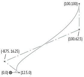
When creating a B-spline, we do not actually need to specify b(t) explicitly — this is automatically constructed to have the required smoothness properties — rather we only need to specify where the knots between the polynomial pieces should be. For the above curve, we want two pieces, one between t=0 and t=0.25, and one between t=0.25 and t=1. To create this B-spline, we would specify the knot vector [0,0,0,0,0.25,1,1,1,1] (when drawing a spline between two fixed endpoints, the first and last knots are always repeated four times to ‘clamp’ the spline to the start and end point). Here is how we could directly define this B-spline in Onshape:

var degree = 3;
var isClosed = false; 
var cpts = [vector(0,0)*meter, vector(12.5,0)*meter,
             vector(-8.75,16.25)*meter, vector(100,62.5)*meter,
             vector(100,100)*meter];
var knots = [0,0,0,0,0.25,1,1,1,1];
var bspline = bSplineCurve(degree, isClosed, cpts, knots);

Note that the control points are not the same as the points you specify to skFitSpline(). In this example, the specified points to skFitSpline() were (0,0), (10,10), (100,100) with startDerivative of (150,0) and endDerivative of (0,150), while the corresponding spline control points are (0,0), (12.5,0), (-8.75,16.25), (100,62.5), (100,100).

When using skFitSpline(), Onshape converts the arguments to B-spline control points, which is easily done with a little mathematics. The first and last fit points become the first and last control points. The second and second-last control points can be calculated from the startDerivative and endDerivative in the same way as we did above for Bézier curves. The other control points can be derived from the remaining fit points with linear algebra (where s(t) = b(t).c).

Conversely, if you want to define a spline using B-spline control points, you can easily convert it to skFitSpline() form by evaluating it at all of its knots, and calculating the startDerivative and endDerivative using the same equations we used above for Bézier curves.

Why B-splines?

It can be seen that the B-spline form of a spline has a number of advantages over specifying polynomial co-efficients for each polynomial piece. Firstly the control points have a more intuitive geometric interpretation than the polynomial co-efficients. Secondly, if b(t) is chosen to have second-derivative continuity, then s(t) automatically has second-derivative continuity without needing to fit a set of co-efficients that satisfy this criterion. However there is nothing magic about B-splines: you can calculate the polynomial co-efficients from the B-spline control points, and vice versa, so they are just different representations of the same curves.

Note also that for a single-piece spline with a simple knot vector like [0,0,0,0,1,1,1,1], b(t) is exactly equivalent to the weighting that defines a Bézier curve, and the resulting spline is the same as the Bézier curve with the same control points. More complicated splines can be decomposed into multiple such Bézier pieces. So again there is nothing more or less powerful about these splines versus a set of Bézier curves joined together; however the B-spline representation requires less control points for the default case that second-derivative continuity is desired.

Directly creating 3D splines in Onshape

There are two FeatureScript functions that can be used for creating splines directly in 3D: opFitSpline() and opCreateBSplineCurve().

opFitSpline() is exactly equivalent to the skFitSpline() function described earlier, except instead of working in the context of a 2D sketch (with an implicit sketch plane), it directly draws a curve in 3D. This can be more convenient than going via a sketch, and the curve need not be constrained to a single plane. The parameters are exactly the same as skFitSpline(), except that all of the points are specified as 3D instead of 2D vectors.

opCreateBSplineCurve() is the most powerful of the spline functions, and also the most daunting. It directly takes a set of B-spline knots and control points. Unlike the other functions, this function lets you create splines of arbitrary degree, not just cubic splines. It also allows you to create closed splines (more on this shortly), and it allows you to create rational splines aka NURBS. I won’t go into rational splines in this article, but they allow you to draw certain curves that wouldn’t otherwise be possible to express in B-spline form.

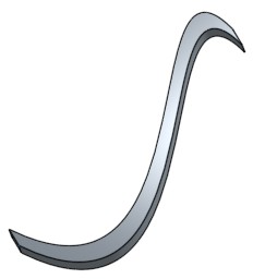
To demonstrate use of these functions, here’s a 3D object that I’ve created by drawing a closed cross-sectional profile with opCreateBSplineCurve() and a guide path with opFitSpline(). I then swept the profile along the guide path with opSweep() and thickened the resulting surface with opThicken() to create a 3D object.

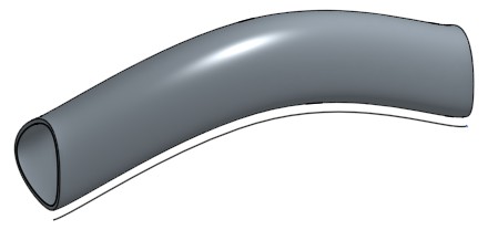
(I’ve left the guide path in the picture for illustration purposes.)

I’m not sure what this object actually is, perhaps it’s a handle for something, or an art piece for my future Onshape museum. But you can see how this might be useful if we need to create a computed surface in an actual engineering problem. Here is the full code:

// cross-sectional profile (closed spline in YZ plane)
// explanation follows after code
var degree = 3;
var isClosed = true; 
var cpts = [vector(0,0,0)*meter, vector(0,-10,30)*meter,
             vector(0,30,10)*meter, vector(0,10,0)*meter];
// repeat first 3 (degree) control points at end
cpts = concatenateArrays([cpts,resize(cpts,degree)]);
var knots = range(0,1,len(cpts)+degree+1);
var bspline = bSplineCurve(degree, isClosed, cpts, knots); 
opCreateBSplineCurve(context, id + "spline1", {
        "bSplineCurve" : bspline 
});

// path for sweep (interpolated spline in XY plane)
opFitSpline(context, id + "spline2", {
        "points" : [
            vector(   0,  0, 0) * meter,
            vector(  50, 20, 0) * meter,
            vector( 100,  0, 0) * meter 
        ],      
        "startDerivative" : vector( 30, 0, 0 ) * meter,
        "endDerivative" :   vector( 30, 0, 0 ) * meter 
});

// sweep spline1 along spline2     
opSweep(context, id + "sweep", {
        "profiles" : qCreatedBy(id + "spline1", EntityType.EDGE),
        "path" : qCreatedBy(id + "spline2", EntityType.EDGE),
        "keepProfileOrientation" : true
});

// thicken to create solid body
opThicken(context, id + "thicken", {
        "entities" : qCreatedBy(id + "sweep", EntityType.BODY),
        "thickness1" : 0 * meter,
        "thickness2" : 1 * meter 
});

// normally we'd delete the sweep path
// opDeleteBodies(context, id + "deletespline2", {
//         "entities" : qCreatedBy(id + "spline2")
// });

One thing that warrants explanation is how I’ve selected the B-spline parameters to create a closed (‘periodic’) spline. For all of the B-splines discussed in part 1, I repeated the first and last knot four times to ensure that the spline passed through the start and end point (the knot sequences looked like [0,0,0,0,0.25,1,1,1,1], for example). In this case, we don’t need or want to clamp the curve to fixed endpoints. Instead, I’ve chosen a uniform set of knots between t=0 and t=1 ([0,0.1,0.2,…,0.8,0.9,1]). The resulting curve does not pass through the first or last control point, but is still guided by the control polygon. I then repeat the first three control points at the end of the list of control points — wrapping part of the control polygon around the curve a second time — which results in a closed spline.

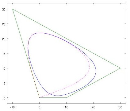
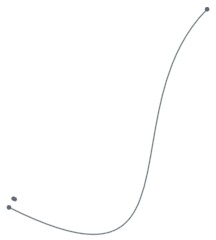
Here is a plot of the spline and control polygon that might help illustrate this. The control polygon starts at the origin (0,0) and goes clockwise around through (-10,30), (30,10), (10,0) and back to (0,0), then retraces (-10,30), (30,10), (10,0). The resulting spline follows the left dotted line from the origin to the top of the egg (from t=0 to t=0.3), traces the egg once (from t=0.3 to t=0.7), and returns to the origin via the right dotted line (from t=0.7 to t=1). When Onshape draws the curve, it only draws the middle part from t=0.3 to t=0.7, so the result is the closed egg shape. (For a spline with degree 3, the outer three knot spans are always ignored when drawing.)

Offset curves

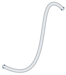
Sometimes it’s necessary to generate a curve that’s “parallel” to another curve, maintaining a constant distance from it. In CAD this is called an offset curve. Here is an example in which I’ve drawn a curve and an offset curve at a given distance. I’ve then used the two curves to create a curved object with constant thickness:

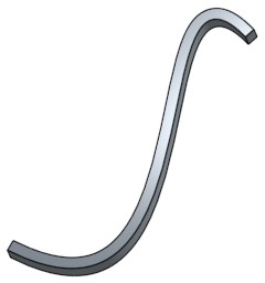
Note that drawing an offset curve is not as simple as translating the curve (moving it in (x,y)). If I was to create this object by copying the bottom curve, dragging the copy towards the top left, and filling in the area between the two, I end up with something that is far from constant thickness:

Rather, to create the offset curve, each point on the curve needs to be moved in a slightly different direction: the direction normal to the curve at that point.

The Onshape sketch GUI has an “offset” tool which makes offsetting a curve easy. I needed to do this programmatically in FeatureScript, though, and there are no documented FeatureScript functions for offset curves. It also turns out that it’s not mathematically possible to express the offset curve in a form that could be input as a new B-spline. So how is Onshape doing this?

Onshape has a handy feature that you can view the code generated by the GUI (right click on a Part Studio → View Code). By perusing the code produced by the offset tool, I did eventually figure out how to create an offset curve from FeatureScript.

Offset curves, using Onshape constraints

The key is to create a new spline using skSplineSegment(), and then add a DISTANCE constraint that constrains it to be a certain distance away from the first spline:

skFitSpline(sketch, "spline1", {
        "points" : [
            vector(0,0) * meter,
            vector(100,100) * meter
        ],
        "startDerivative" : vector(300,-150) * meter,
        "endDerivative" : vector(150,-150) * meter
});
skSplineSegment(sketch, "spline2", {});
skConstraint(sketch, "distance", {
        "constraintType" : ConstraintType.DISTANCE,
        "localFirst" : "spline1",
        "localSecond" : "spline2",
        "length" : 5 * meter,
        "direction" : DimensionDirection.MINIMUM,
        "alignment" : DimensionAlignment.ANTI_ALIGNED
});
// not strictly required?
skConstraint(sketch, "offset", {
        "constraintType" : ConstraintType.OFFSET,
        "localMaster" : "spline1",
        "localOffset" : "spline2"
});

The OFFSET constraint does not seem to be required for the solver to do the right thing here, it may just be for GUI display purposes, but I’ve left it in the code example just in case.

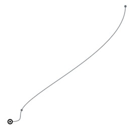
There is one oddity with this. We have not specified any constraints on the endpoints, and sometimes the solver takes more liberty with the second endpoint than you might like. For example, depending on spline parameters, you can get something like this:

I’ve not been able to figure out the logic of how the solver chooses the second endpoint, however this is of purely academic interest — in practice, the requirements of the CAD problem will usually dictate physical constraints on the endpoints. If you want to force the second curve to end at the same point as the first curve, you can add an extra constraint between the endpoints, for example:

skConstraint(sketch, "distance.end", {
        "constraintType" : ConstraintType.DISTANCE,
        "localFirst" : "spline1.end",
        "localSecond" : "spline2.end",
        "length" : 5 * meter,
        "direction" : DimensionDirection.MINIMUM,
        "alignment" : DimensionAlignment.ANTI_ALIGNED
});

In the earlier picture where I used an offset spline to create a 3D object, I needed to join the spline ends with two line segments to form a face. As in the sketch GUI, this can be done by using COINCIDENT constraints. (The code is simple but rather verbose; if you need many such constraints in your FeatureScript it may be worth writing a makeCoincident() function.)

skLineSegment(sketch, "line1", {});
skConstraint(sketch, "coincident.line1.start", {
        "constraintType" : ConstraintType.COINCIDENT,
        "localFirst" : "line1.start",
        "localSecond" : "spline1.start"
});
skConstraint(sketch, "coincident.line1.end", {
        "constraintType" : ConstraintType.COINCIDENT,
        "localFirst" : "line1.end",
        "localSecond" : "spline2.start"
});
skLineSegment(sketch, "line2", {});
skConstraint(sketch, "coincident.line2.start", {
        "constraintType" : ConstraintType.COINCIDENT,
        "localFirst" : "line2.start",
        "localSecond" : "spline1.end"
});
skConstraint(sketch, "coincident.line2.end", {
        "constraintType" : ConstraintType.COINCIDENT,
        "localFirst" : "line2.end",
        "localSecond" : "spline2.end"
});

The sketch GUI also has a “slot” tool that allows you to conveniently draw two offset curves, with semicircular end caps. This can be implemented in FeatureScript following the same approach as the above code, replacing skLineSegment() with skArc(); indeed under the bonnet this is what the slot tool generates.

Offset curves in Onshape

While we can now create an offset curve in a sketch, we still haven’t really answered the question of how Onshape is doing this magic. Have the wizards at Onshape cracked the problem of how to derive offset spline parameters from the original spline?

While their wizardry is impressive, the answer is no, Onshape actually uses a much simpler method. It stores an offset curve as the original spline parameters and an offset value. The points of the offset curve can then be calculated numerically at evaluation time.

Unfortunately, there does not seem to be any way (that I can find) to specify the offset value explicitly when creating a spline. For splines used in sketches, you can use a DISTANCE constraint as shown above, and the solver will assign the right offset to the second spline. This is a little tedious but works well. However it can’t be applied to splines created outside of sketches (opFitSpline() or opCreateBSplineCurve()); in this case there is no way that I can find to specify the offset value. I hope that the ability to specify an explicit offset might be added in a future version.

Side note on Onshape rendering

As a side note, while the Onshape computational engine evaluates curve points precisely where needed, the objects displayed in the GUI are built using straight edges. The rendering is not refined as you zoom in. Thus, attempting to visually place elements may produce unexpected results. For example, below is a line segment that is constrained to be co-incident with an spline; in the zoomed-in GUI, there is a gap you could drive a large bacterium through. The line segment does, however, touch the real spline.

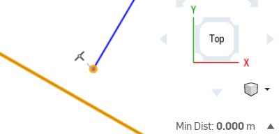
For the most part the accuracy of the GUI approximation is a moot point of course. The underlying solver does evaluate the points precisely, and the generated geometry is correct. The take home message is that — as in any parametric CAD system — you should specify any constraints that you need and not rely on visual placement in the GUI.

Offset curve self-intersection

When drawing offset curves on the concave side of a spline, there is a problem that sometimes arises: the offset curve may run into itself (in fact, this always happens for some offset distance, but it’s most problematic when the spline has high curvature). If we blindly plot the curve that results, we see that the offset curve has a loop:

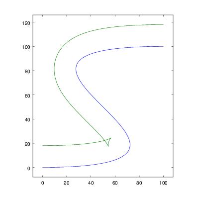
(If you’re surprised by the shape of this loop, take something like an eraser and sweep it along the path; there is a point where the top of the eraser has to start moving in the other direction to make it around the tight bend.)

In this case, Onshape throws up its hands and refuses to create the offset curve. Sometimes this can happen even when one is not explicitly working with offset curves: for instance, the “thicken” operation I used earlier in this article requires the calculation of offset curves, which may fail depending on the thickness value. In that example, a value of 1 meter works okay, but 2 meters fails (in either direction), and it’s not immediately obvious where in the curve the self-intersection is.

There do exist algorithms that can trim loops from offset curves. Even after trimming the loop, there is still the complication that there is a cusp (vertex) in the curve where the loop was, which changes the geometry of any objects built from this curve: for example, if you were to extrude the above curve, there is now an extra edge in the knee. I’ve noticed that Onshape refuses to draw splines with cusps, which is likely to avoid this problem of surplus geometry. One way around this would be to interpolate an arc at the cusp, but this clearly involves a lot of added complexity in the computation.

I do hope that Onshape considers supporting some form of offset curve trimming in the future, as well as improving robustness with respect to cusps and other geometry anomalies. While often you do want to know about these anomalies, the current behaviour — where parts can suddenly fail to render after making small changes to parameters — can be quite frustrating when trying to fine-tune your designs.

Wrapping up

This article involved a bit of a ‘deep dive’ into splines and offset curves, and how to work with them in FeatureScript. I learned a lot in the process, and hopefully this will help you too if you find yourself needing to create complex curved objects. Happy designing!