Electromagnetic radiation from accelerating charges

Electromagnetic radiation is something that has often eluded my intuition. Electrical engineering depends on numerous abstractions: current flowing in wires like a fluid, capacitance/inductance in lieu of near field interactions, antenna theory to model far field interactions, etc. These abstractions are essential to make electromagnetic theory tractable for everyday use. But they also obscure the underlying physics and can result in incorrect conclusions when reality crosses the boundaries of the abstractions.

Looking at electromagnetic radiation from first principles provides, I think, some interesting insights. In this blog post I show how the phenomenon of radiation can be derived from little more than basic special relativity (which itself follows from only a small number of postulates about the universe). This is not new but I think many readers may not be aware of it.

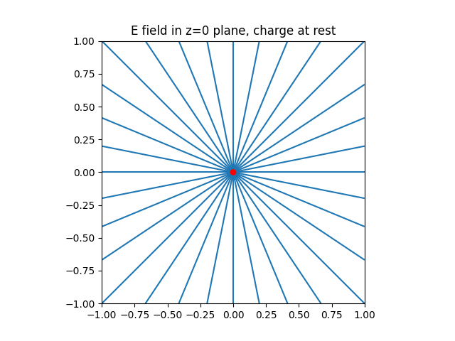
Case 1: charge at rest

First consider a charge at rest for all time (in some chosen reference frame). It has a spherically symmetric electric field that follows Coulomb’s law. We know this from basic high school physics but also it should be clear from the geometrical symmetry of the situation.

Case 2: charge moving at constant velocity

Next, consider a charge with constant velocity along the x axis for all time (in some chosen reference frame). Observers co-moving with the charge cannot tell the difference from the situation in case 1 and must, by the principle of relativity, see the spherically symmetric Coulomb field. To determine what is seen by observers in the reference frame where the charge is moving, we must apply a coordinate transformation consistent with special relativity (Lorentz transformation). The result is the following slightly squashed field pattern:

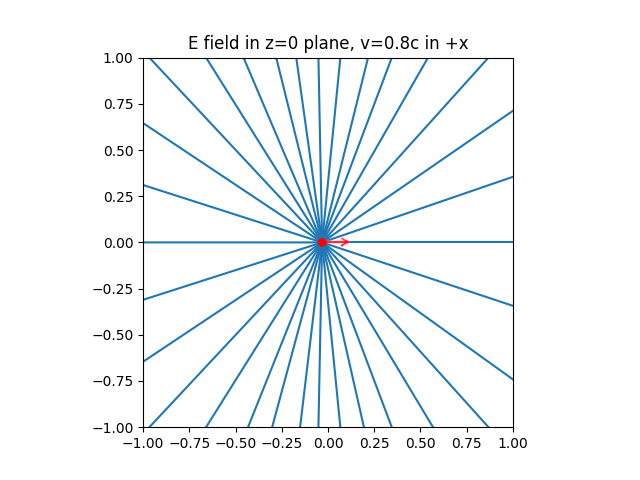
There are three things to note:

1. The field pattern is squashed in the x axis due to the coordinate transformation (‘length contraction’). I have exaggerated this here by plotting at v=0.8c, but this effect will happen to a small degree at any velocity.
2. Additionally, the y and z components of the E-field are amplified due to how the electromagnetic field tensor transforms between the two reference frames (E’_y = γE_y, E’_z = γE_y). This provides an extra squashing of the field pattern.
3. The field lines appear to radiate from the instantaneous position of the charge. I will discuss this anomaly more later in this post.

Putting things together: accelerated charge

Now consider what happens if we combine both plots, introducing time: we start a charge at rest and accelerate it to some constant velocity. Below is an animation I generated using a simple Python program (press play to run the video). This was inspired by Teviet Creighton’s excellent animation but, not having a copy of the code, I re-invented the wheel.

First consider the outside of the plot. Observers that are more than ct distance away from the origin (that is, outside the light cone of the point (0,0,0,0)) have not have not seen the charge start moving yet, so they must still observe the original spherically-symmetric Coulomb field.

Meanwhile, the field in the middle of the plot is the distorted field of a charge moving at constant velocity.

In between, we need to join up those field lines. There are no sources/sinks in this region so we know that the field lines must be contiguous. Furthermore, the charge couldn’t have instantaneously accelerated from stationary to constant velocity, so the transition from one region to the other must happen continuously over some finite time, with a shape that depends on the acceleration profile.

This boundary layer — that expands outwards at the speed of light — is an outgoing wave packet. Notice that the electric field lines here are largely transverse. Additionally (not drawn here), there is a magnetic field consistent with the rightward velocity of the charge, that is pointing out of the page above the x axis and into the page below the x axis [assuming a positive charge]. With some additional curling of your right hand, you can see that the Poynting vector is indeed outwards everywhere.

Notes on the code

The Python code I wrote to generate the above animation (download) evaluates the electric field at any point directly using equation 14.14 from Jackson’s Classical Electrodynamics (3rd Ed), also given on the Wikipedia page for Liénard–Wiechert potential. This equation describes the field from a point charge and can be derived (not painlessly) from the Liénard-Weichert potentials. I take c=1 (natural units) and ignore scaling constants.

The only complicated part is evaluating the retarded time at which a wavefront observed at a particular (x,y,0,t) was emitted by the source. In the constant velocity region, this involves a quadratic equation. In the constant acceleration region, this involves a (depressed) quartic equation. In my simple case, I evaluate both using formulas rather than numerical methods to minimise numerical error.

The field lines are drawn using a Runge-Kutta method: start at some point, evaluate the E-field, then take a small step in that direction. This makes physical sense as electric field lines reflect the path that would be taken by a test charge.

My favourite trick is this: to draw the field lines, I trace them outside-in (from the boundary) rather than inside-out (from the charge). At r>ct, we know that the field is uniform so we can start from uniformly distributed starting points anywhere outside this shell.

My first few versions of the code started from the charge and traced outwards, but this requires more complex code to choose start points for the radial field lines around the charge. (Around the moving charge the field lines are not equally distributed, instead they must be drawn so as to subtend equal fluxes.) Also integrating outwards means that any numerical error results in obvious wobbly lines (close to the axes where this is obvious to the viewer), while integrating inwards produces a smoother video.

Charge moving at constant velocity, revisited

I noted above that, when evaluating the field of a charge moving at constant velocity, field lines appear to radiate from the instantaneous position of the charge. An observer who is a light second away sees an electric field direction that is consistent with the current position of the charge, and not where the charge was a second ago.

This is surprising and raises the spectre of faster-than-light propagation, but note that there is no new information being conveyed by a charge that is moving at constant velocity. Feynman says, “nature seems to be attempting to guess what the field at the present time is going to be, by taking the rate of change and multiplying by the time that is delayed” [Feynman Lectures on Physics, 28-1]. The idea of nature ‘attempting to guess’ the future field does not really sit well with me or give me much physical intuition. But consider what the electric field would look like if it reflected where the particle was at the past (‘retarded’) time:

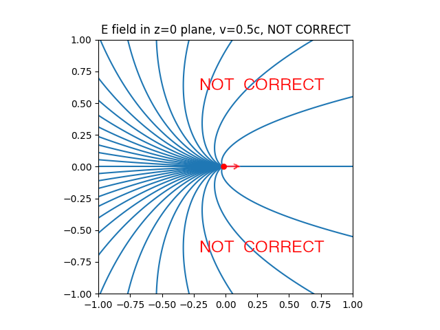
In this case we would end up with a very strange transformation between this observed field and the one in the charge’s reference frame: one that is not a simple reference frame transformation but must depend on the position of the charge. So we must accept something that seems counter-intuitive to make the rest of the physics simple and consistent.

Final thoughts

Consider now any electronic system. If charges travel with constant velocities, there is no new information conveyed. Any computation or communication must involve acceleration of charges. Any acceleration of charges produces electromagnetic radiation, theoretically out to infinity.

In practice we mitigate this by ensuring that nearby charges accelerate in opposite directions, so that that the radiated waves interfere destructively (keeping ‘inductive loop area’ small, differential signalling, etc.). But because these waves are emanating from separate centers and travelling outwards exactly at the speed of light, they can never cancel exactly at all points in space. Thus it is not possible to design a useful circuit that doesn’t radiate at all, or conversely (by the reciprocity principle) a useful circuit that is not affected by electromagnetic interference.

Fortunately for information security, at some small distance it becomes impractical to recover information about individual charge accelerations, due to noise, EM field quantization and interaction with other matter. But in some theoretical sense, information about every charge acceleration is inescapably encoded in the radiated electromagnetic field, which is a fascinating thought.