
 BETA
BETAIn part 1, we introduced the reverse sprinkler problem and attacked the most ideal case, ignoring factors such as pipe diameter. Now we will perform a more general analysis.
A theorem
Consider any two closed surfaces in a fluid, one wholly inside the other, with a solid in the middle:
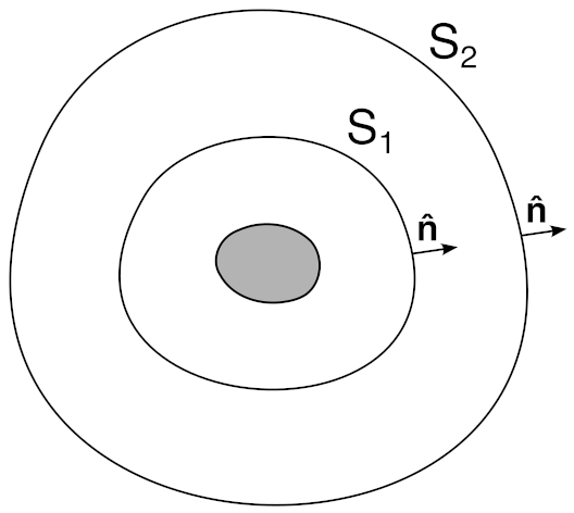
Eventually we will place the sprinkler in the center but at this stage the treatment is more general.
We assume that the fluid is incompressible, body forces like gravity can be ignored, and that steady state flow has been reached for practical purposes. Applying the Reynolds transport theorem for linear momentum for the control volume bounded by S1 and S2, we can write down the following (as in part 1, we drop terms with time derivatives due to the steady state assumption):
![\[\oiint_{S_2} \boldsymbol{\sigma}\cdot\mathbf{\hat{n}} \mathop{dA} - \oiint_{S_1} \boldsymbol{\sigma}\cdot\mathbf{\hat{n}} \mathop{dA} = \rho\oiint_{S_2} \mathbf{\vec{v}} (\mathbf{\vec{v}}\cdot\mathbf{\hat{n}}) \mathop{dA} - \rho\oiint_{S_1} \mathbf{\vec{v}} (\mathbf{\vec{v}}\cdot\mathbf{\hat{n}}) \mathop{dA}\]](https://zmatt.net/wp-content/ql-cache/quicklatex.com-0e8cae82a107b1c4b04ea84db2749486_l3.png "Rendered by QuickLaTeX.com")
where:
- σ is the stress tensor at each point, including the effects of both hydrostatic pressure and viscous stress,
- n̂ is the outwards-pointing surface normal at each point,
- ṽ is the fluid velocity at each point,
- ρ is the fluid density, assumed constant, and
- dA is a surface area element.
Put in plain language, in steady state, any change in momentum due to stresses on the control volume between S1 and S2 (the left side of the equation) must equal the momentum carried out of the control volume by fluid velocity (the right side of the equation). Otherwise this area of space would be gaining momentum, contradicting the steady state assumption.
Rearranging this to put the terms for each surface together:
![\[\oiint_{S_2} \boldsymbol{\sigma}\cdot\mathbf{\hat{n}} \mathop{dA} - \rho\oiint_{S_2} \mathbf{\vec{v}} (\mathbf{\vec{v}}\cdot\mathbf{\hat{n}}) \mathop{dA} = \oiint_{S_1} \boldsymbol{\sigma}\cdot\mathbf{\hat{n}} \mathop{dA} - \rho\oiint_{S_1} \mathbf{\vec{v}} (\mathbf{\vec{v}}\cdot\mathbf{\hat{n}}) \mathop{dA}\]](https://zmatt.net/wp-content/ql-cache/quicklatex.com-0e7a1759cfa29c0024bf665f26bed95a_l3.png "Rendered by QuickLaTeX.com")
This must be true for any pair of surfaces we choose in the fluid, which can only be true if this is a constant. I will call this closed-surface momentum flux F̃ for reasons that will become apparent in a second.

If there is nothing inside S1, then we can shrink S1 to a point and conclude that F̃ = 0. If there is a rigid object inside S1, then we can shrink S1 to the object boundary and F̃ is the net force on the object (there is no convective momentum flux into a rigid object, so only the stress terms remain). Now of course, if F̃ turns out to be non-zero, the object would start to move; for this analysis we assume that it could be held by a body force of some sort, and we do not attempt to shrink the surface into the solid part of the object.
Applying the Reynolds transfer theorem for angular momentum, we arrive at corresponding expressions for angular momentum flux and hence torque. This is a little less intuitive than the linear momentum case, but the expressions are exactly analogous.

Back to the sprinkler problem
Let us return to the sprinkler problem and apply the above insights. We take in particular a surface S2 approaching infinity, and a surface S1 hugging the sprinkler.
To visualize the flow near infinity, we zoom out, and out, and out on the problem. Eventually the scale of the sprinkler is negligible with respect to the scale we are considering, and what we have looks like a point pressure sink. Therefore we can reasonably assume that the flow at sufficient distance approaches a flow that is radially inwards. A visualization of this is shown below (here velocity contours are shown; similar arguments can be made for the pressure field):
By symmetry then, the momentum flux and stress integrals approach zero as the radius approaches infinity, and both F̃ = 0 and τ̃ = 0 when evaluated on S2.
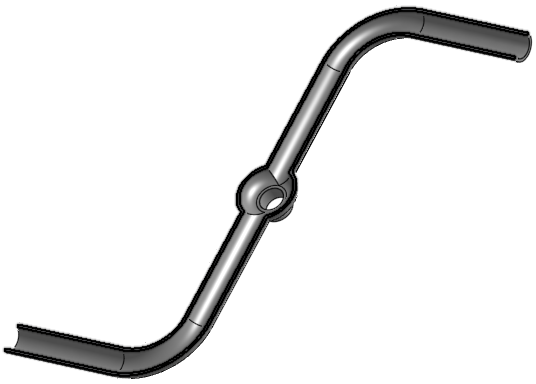
We assume that the sprinkler consists of a rigid rotating body, coupled via a rotary bearing to a stationary base. We assume that we can ignore the base for this treatment and focus on the rotating part. Here is a cross-sectioned view of the body under consideration, showing an outlet at the bottom of the rotating body:
We now construct a surface S1 as follows. Choose a surface around the rotating body of the sprinkler and shrink wrap the sprinkler, then keep sucking the surface into the sprinkler arms until S1 covers all surfaces of the rotating body or touches itself. At the bottom of the hub the control surface spans the outlet, from both sides. (The outlet is shown in pink since it is below the plane of the cross-section.)
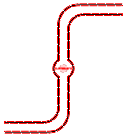
Where the surface S1 touches itself, it always has zero integrals due to opposite normals on the two sides. We make an exception for the outlet and insert a magic pressure source between the two sides, since this is where some apparatus would provide suction. Thus we have two relevant parts to the surface: the outlet, and the rest of the surface which is in contact with the sprinkler.
By the theorem demonstrated earlier in this post, the total angular momentum flux integral over surface S1 is zero, since it is zero over S2. However, considering the pieces of S1, there is no physical reason that the integral must be zero over the outlet, and in fact in general it is not. In this case we know that an equal-and-opposite torque has been imparted to the sprinkler via the stresses on the surface.
A note on the forward sprinkler case
It might seem that we can apply the same argument to the forward sprinkler, but we cannot. The forward sprinkler has an outwards jet which carries momentum outwards, and so the integral over any S2 is non-zero. In the presence of viscosity the jet diffuses, but still in theory momentum is carried to infinity. Of course in the real world the outgoing momentum does eventually hit a wall or dissipate beyond detection, but these effects are outside the model that we are applying.
Discussion
We have come what may seem the long way around to say this: subject to certain assumptions that will be expounded below, there is no angular momentum exchanged with the surrounding fluid, and so there is no rotation attributable to the sucking of fluid into the sprinkler. However, if the fluid flowing through the sprinkler gains a non-zero net angular momentum, and ‘leaks’ this angular momentum from the rotating part to the stationary part (and thence to the attachment point or efflux tank), then the sprinkler must rotate to globally conserve angular momentum.
This result is powerful and yet difficult to apply, since it does not directly tell us the torque for a particular design. A weaker version that we will make use of in our part 3 analysis involves pulling back the control surface to given planes within the arms:
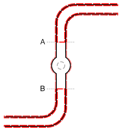
If we can ignore the stresses on the pink parts of the exterior surface, then we can say that the torque acting on the ends of the arms (beyond the chosen transection planes A and B) is the negative of the angular momentum flux in the fluid through those transection planes. As we will see, the error in this approximation is negligible unless the chosen planes are close to the end of the arms.
Let us be explicit about our assumptions:
- We have assumed that the fluid domain is unbounded and there is no wall. In any real experiment or even computer simulation, there will be some sort of boundary, and this can produce a weak force towards the walls, consistent with “vacuum cleaner” intuition. However unless the walls are close to the inlets, this effect is very weak, and will not be significant in the torque analysis (see part 3 of this series).
- We have assumed that we can ignore the effect of the stationary base and any other experimental apparatus on the fluid flow. Again, the stationary base is usually far enough from the inlets for any effect to be negligible.
- We have assumed that we can perform the analysis at steady state with the sprinkler held in position, and then extrapolate the expected rotation from the torque felt on the stationary sprinkler. Thus:
- It ignores any non-steady-state effects, for example many experiments have shown that there is a brief angular impulse as suction is applied to the sprinkler, and similarly a brief angular impulse as suction is removed from the sprinkler (the pressure changes cannot propagate instantaneously).
- It ignores the effects of actual rotation on the fluid flow. However, intuitively, rotation will introduce drag forces, it should not positively increase the thrust force, otherwise we would have a sort of perpetual motion machine.
- We have assumed negligible dissipation in the fluid. Dissipation can convert macroscopic momentum into microscopic momentum (e.g. thermal motion of molecules), in which case macroscopic momentum may not be perfectly conserved.
In part 3, the final part, we will make this more concrete by performing some simulations and analyzing the results.
