The physics of toppling dominoes

This post has an accompanying YouTube video here.

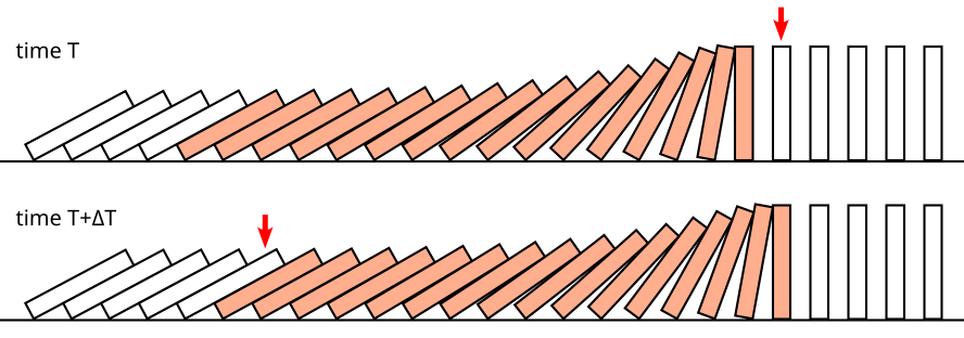
Most people think of toppling dominoes as a sequential chain reaction where one domino falls, then the next, then the next. But consider this picture of a domino line toppling:

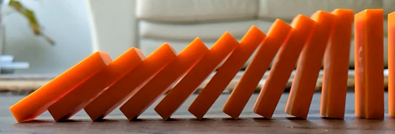
The dominoes do not fall one by one, they stack together as they fall. Each domino leans on the next domino which leans on the next and so on. The stacked dominoes push on the domino at the head of the line, resulting in a domino wave front that travels much faster and more reliably than if each domino just bumped the next domino and retired from the picture.

In this post, I will show how to derive equations of motion for a line of dominoes, from which we can build a domino simulation program. The resulting Python code is available on github here. I will also look at the velocity of the domino wave front, and how we can derive back-of-the-envelope expressions for its velocity.

Most of the derivations here are not novel, the arguments are similar to those made by van Leeuwen (2004) and Shi (2019). However, I have worked through the problem myself and tried to present it as logically as possible. In my opinion my velocity expressions have some advantages over those presented in the previous literature.

Setup

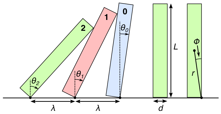
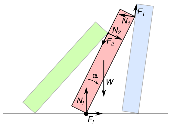
The following figure defines the basic geometry and symbols that I will use. Frustratingly every author in this field uses slightly different conventions, so care needs to be taken when comparing different sources.

I will make the assumptions that:

There is sufficient friction with the floor that the dominoes do not slide.
The dominoes do not rotate in any axis other than the one corresponding to forward toppling.
Each falling domino ends up leaning on the next one a short time after collision.

In fact, these are the only assumptions we need to make to solve the problem. They are actually quite well satisfied in most real life situations, with only minor deviations. I will revisit these assumptions at the end.

Angles, velocities and accelerations

It should be evident from the figure above that we can calculate the angles θ₁, θ₂, etc. of each of the stacked dominoes for any given angle of the leading domino θ₀, as a “simple” matter of geometry. The following recursive relation can be derived:

(1) $\begin{equation*} \sin(\theta_i-\theta_{i-1}) = \left(\frac{\lambda}{L}\right) \cos(\theta_{i-1}) - \left(\frac{d}{L}\right) \end{equation*}$

Differentiating this equation with respect to time and rearranging, it follows that we can also recursively express the angular velocity of any stacked domino:

(2) $\begin{equation*} \frac{\dot\theta_i}{\dot\theta_{i-1}} &= 1 - \left(\frac{\lambda}{L}\right)\frac{\sin(\theta_{i-1})}{\cos(\theta_i-\theta_{i-1})} \end{equation*}$

We will call this ratio $\Omega_i$ . Differentiating again, we can recursively express the angular acceleration of any stacked domino:

(3) $\begin{align*} \ddot\theta_i &= \Omega_i\ddot\theta_{i-1} + \Psi_i\dot\theta_{i-1}^2 \\ \text{where } \Psi_i &= - \left(\frac{\lambda}{L}\right)\frac{\cos(\theta_i) + \sin(\theta_{i-1})\sin(\theta_i-\theta_{i-1})\Omega_i}{\left(\cos(\theta_i)-\cos(\theta_{i-1})\right)^2} \end{align*}$

So, under the assumptions, it is only the leading domino that is “free”, and the motion of all other dominoes can be calculated from it. Let us focus then on how to determine the motion of the leading domino.

Two phases

There are two phases in the motion of the leading domino:

The acceleration phase: the leading domino accelerates under the combined influence of gravity and the normal force from previous dominoes.
The collision phase: the leading domino hits the next domino, providing an “initial velocity” to the next domino. We will find that there is only one value for this velocity that is possible under assumptions 1-3. Now the new domino becomes the leading domino and we return to phase I.

Phase I: acceleration phase

Ignoring friction for now, energy is conserved in this phase: the potential energy of the falling domino train turns into kinetic energy. However, it is not true to say that a given domino’s potential energy turns into kinetic energy in the same domino. The ratios of domino velocities are constrained as shown above in equation (2). The following figure shows how potential energy (blue and cyan bars) and kinetic energy (red bars) change during a particular acceleration phase, i.e. since the previous collision:

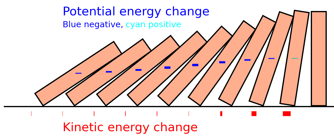
It can be seen that the middle dominoes in this group have fallen the most during this time, but the energy has mostly been transferred to the front of the train. In fact, the leading domino has gained potential energy; this is because its center of mass needs to travel upwards slightly for it to tip over, and depending on the domino spacing, this can be the case for most or all of the leading domino’s acceleration phase.

We can derive the equations of motion in various ways. Using Lagrangian mechanics is tempting here, since under our assumptions, the configuration space of the system can be defined by only one generalized coordinate (θ₀, the angle of the leading domino). However, the Newtonian method of forces ends up being preferable when considering friction and collision dynamics. I will present both methods here; feel free to skip the Lagrangian derivation if it is daunting, but I do find it quite elegant.

Lagrangian method

The potential energy of the domino system can be expressed as follows, taking the zero point as the floor:

$\begin{align*} V &= mgr \cos(\theta_0-\phi) + mgr \cos(\theta_1-\phi) + mgr \cos(\theta_2-\phi) + ... \\ &= mgr \sum_{k=0}^{n} \cos(\theta_k-\phi) \end{align*}$

Notice that for each domino, there is $mgr \cos(\theta_k-\phi)$ rather than $mg\tfrac{L}{2}\cos(\theta_k)$ , this reflects the fact that each domino pivots around its corner and its center of mass must actually be lifted slightly until the tipping point at angle Φ. (Other sources write the potential energy as $mg\tfrac{L}{2}\cos(\theta_k)+mg\tfrac{d}{2}\sin(\theta_k)$ , but I prefer the version with Φ as it reduces the number of trigonometric functions.)

The kinetic energy of the domino system can be expressed as a sum of rotational kinetic energies, as follows:

(4) $\begin{align*} T &= \tfrac{1}{2}I\dot\theta_0^2 + \tfrac{1}{2}I\dot\theta_1^2 + \tfrac{1}{2}I\dot\theta_2^2 + ... \\ &= \tfrac{1}{2}I\dot\theta_0^2 + \tfrac{1}{2}I\dot\theta_0^2\left(\frac{\dot\theta_1}{\dot\theta0}\right)^2 + \tfrac{1}{2}I\dot\theta_0^2\left(\frac{\dot\theta_1}{\dot\theta0}\right)^2\left(\frac{\dot\theta_2}{\dot\theta1}\right)^2 + ... \\ &= \tfrac{1}{2}I\dot\theta_0^2 K(\theta_0) \quad\text{where } K(\theta_0) = \sum_{k=0}^{n} \prod_{j=1}^{k} \Omega_j(\theta_0)^2 \end{align*}$

We have defined a function K which is the ratio of the kinetic energy of the entire domino train to the kinetic energy of the first domino, this will turn out to be a useful quantity throughout. Note that K is a function of θ₀, a fact which will become important in a moment (it is also technically a function of the number of dominoes n, but we assume this is constant during the acceleration phase).

So the Lagrangian is:

$\begin{align*} L &= T-V \\ &= \tfrac{1}{2}I\dot\theta_0^2 K(\theta_0) - mgr \sum_{k=0}^{n} \cos(\theta_k-\phi) \end{align*}$

Now we apply the Euler-Lagrange equation, as usual when crunching through Lagrangian mechanics problems. However since K is a function of θ₀, there are two complications which may catch out the novice Euler-Lagrangist. Firstly, the $\frac{\mathrm{d}}{\mathrm{d}\theta_0}$ term ends up capturing the kinetic energy term, unlike some simpler problems where it is purely the derivative of the potential energy. Likewise, even though K is a constant when taking $\frac{\mathrm{d}}{\mathrm{d}\dot\theta_0}$ , the total derivative $\frac{\mathrm{d}}{\mathrm{d}t}$ must include the time derivative of K(θ₀). Thus:

$\begin{align*} \pdv{L}{\theta_0}-\odv*{\left(\pdv{L}{\dot\theta}\right)}{t} &= 0 \\ \tfrac{1}{2}I\dot\theta_0^2 K'(\theta_0) + mgr \sum_{k=0}^{n} \sin(\theta_k-\phi) \odv{\theta_k}{\theta_0} - \odv*{\left(I\dot\theta_0 K(\theta_0)\right)}{t} &= 0 \\ \tfrac{1}{2}I\dot\theta_0^2 K'(\theta_0) + mgr \sum_{k=0}^{n} \sin(\theta_k-\phi) \odv{\theta_k}{\theta_0} - I\ddot\theta_0 K(\theta_0) - I\dot\theta_0 \dot{K}(\theta_0) &= 0 \\ mgr \sum_{k=0}^{n} \sin(\theta_k-\phi) \odv{\theta_k}{\theta_0} - I\ddot\theta_0 K(\theta_0) - \tfrac{1}{2} I\dot\theta_0^2 K'(\theta_0) &= 0 \end{align*}$

Where I use $K'$ to mean $\frac{\mathrm{d}K}{\mathrm{d}\theta_0}$ and $\dot{K}$ to mean $\frac{\mathrm{d}K}{\mathrm{d}t}$ , and I use the substitution $\dot{K} = K'\dot\theta_0$ which is more obvious when written as $\frac{\mathrm{d}K}{\mathrm{d}t} = \frac{\mathrm{d}K}{\mathrm{d}\theta_0}\cdot\frac{\mathrm{d}\theta_0}{\mathrm{d}t}$ . Now rearranging for the angular acceleration:

(5) $\begin{align*} \ddot\theta_0 &= \frac{mgr \sum_{k=0}^{n} \sin(\theta_k-\phi) J_k(\theta_0) - \tfrac{1}{2} I\dot\theta_0^2 K'(\theta_0)}{I K(\theta_0)} \\ & \qquad \text{where } J_k(\theta_0) = \odv{\theta_k}{\theta_0} = \frac{\dot\theta_k}{\dot\theta_0} = \prod_{j=1}^{k} \Omega_j(\theta_0) \end{align*}$

This may look complex but it’s easy enough to evaluate in numerical simulation: given some start angle $\theta_0$ and initial angular velocity $\dot\theta_0$ , we obtain the corresponding angular acceleration from this equation, which we use to update the $\theta_0$ and $\dot\theta_0$ for the next timestep (either by simple Euler stepping or by using a higher order method like Runge-Kutta)¹.

Newtonian method

As usual in Newtonian mechanics, the first step here is to draw a free body diagram for one of the dominoes. W is weight, N_f is the floor normal force, F_f is floor friction, N₁ and N₂ are the normal forces with neighbouring dominoes (with moment arms a₁ and b₂ respectively), and α is the resulting acceleration:

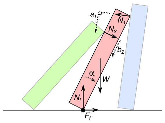
Now we can write three Newton-Euler equations (F=ma horizontally and vertically, and τ=Iα rotationally). Actually we need not write down the two force equations at this point, we can use them to evaluate F_f and N_f once we have the other variables solved. For the torque around the rotation axis (the bottom right of the domino), we have:

(6) $\begin{align*} a_1 N_1 - b_2 N_2 &- r\sin(\theta_1-\phi)W = -I\alpha \\[3pt] \text{where } a_i &= L\cos(\theta_i-\theta_{i-1}) \\ b_i &= L\cos(\theta_i-\theta_{i-1})-\lambda\sin(\theta_{i-1}) \end{align*}$

Note that even though the rotation axis is not the center of mass, it is fixed so there is no fictitious torque term required. The right hand side is negative as I wrote this equation using the standard right-hand-rule convention to avoid confusion, and α is defined oppositely. θ₁ is the lean angle of the red domino and θ₀ is the lean angle of the blue domino, as defined in the earlier geometry diagram.

For the whole domino system, we then have a matrix of equations as shown below. Each domino’s acceleration α_n can be expressed as a linear function of the previous domino’s acceleration, as shown in equation (3), so all accelerations can be written as c_nα₀ + d_n for some constants c_n, d_n:

$\begin{alignat*}{4} & b_1 N_1 &- r\sin(\theta_0-\phi)W &= -I\alpha_0 \\ a_1 N_1 -& b_2 N_2 &- r\sin(\theta_1-\phi)W &= -I(c_1\alpha_0 + d_1) \\ a_2 N_2 -& b_3 N_3 &- r\sin(\theta_2-\phi)W &= -I(c_2\alpha_0 + d_2) \\ && ..&. \\ a_n N_n &&- r\sin(\theta_n-\phi)W &= -I(c_n\alpha_0 + d_n) \end{alignat*}$

We have N equations and N unknowns (N-1 normals and the acceleration α₀), so this system can be solved. For example, we can rearrange each equation into the form N_n+1 = Cα₀ + D and substitute into the next equation, the last domino has no second normal force so α₀ is obtained from the final equation.

Once we have a method for solving for α₀ (= $\ddot\theta_0$ ), we can simulate the acceleration phase iteratively as described at the bottom of the previous section. Ultimately the solution of this equation set must be the same as that given by the Lagrangian method, although that is not easy to arrive at from here.

Newtonian method with domino-domino friction

We have already included floor friction in the above models, as it is necessary for the dominoes not to slide, which is one of our assumptions. However, we have not included friction between dominoes. Below is a new free body diagram with domino-domino friction F₁ and F₂ included:

Because of the constrained motion of the dominoes, we know that the stacked dominoes are always sliding. Thus we know that the friction force in each case is F = μN with μ being the dynamic co-efficient of friction (and not the static case F ≤ u_sN which would make the problem more difficult). We also know the direction of the friction forces, which are as shown.

The new torque equation is as follows:

$\begin{align*} a_1 N_1 + \mu L \sin(\theta_i-\theta_{i-1}) N_1 - b_2 N_2 + \mu d N_2 &- r\sin(\theta_i-\phi)W = -I\alpha \end{align*}$

We can absorb the friction terms into the coefficients for N₁ and N₂, resulting in:

(7) $\begin{align*} A_1 N_1 - B_2 N_2 &- r\sin(\theta_i-\phi)W = -I\alpha \\[3pt] \text{where } A_i &= a_i + \mu L \sin(\theta_i-\theta_{i-1})\\ B_i &= b_i - \mu d \end{align*}$

This is now the same form as equation (6) in the previous section, with a_n replaced by an “effective moment arm” A_n and b_n replaced by an effective moment arm B_n. Then we have exactly the same problem and solution method as in the previous section, only with changed coefficients.

Phase II: collision phase

In this phase, the leading domino collides with the next domino, and in this process some kinetic energy may be lost (actually, we know for a fact that some kinetic energy is lost, since toppling dominoes produce satisfying clacking sounds). We must decide on a “collision law” that dictates the various velocities after the collision.

It is very tempting to assume conservation of angular momentum within the domino system, and some previous authors have fallen into this trap. For a single domino, the reaction forces at the floor (normal force and friction force) act through the pivot point, and therefore do not affect the angular momentum of the domino around that point. For multiple dominoes however, we must calculate the system angular momentum around a single point, and not around a different point for each domino! It is clear then that the floor reaction forces cannot be ignored, and the domino system angular momentum can and likely does change during a collision.

How should we model the collision then?

As is often the case in collision modelling, we assume that the collision occurs over a negligibly short period of time. Thus we can ignore acceleration due to gravity during this time, and simply consider the angular impulses given to each domino, which must be such that:

the final velocities satisfy the usual recurrence relation, equation (2), and
the final velocities are possible to achieve using a physically transmissible set of forces that satisfy the relationships in our previous Newton/Euler analysis, ignoring gravity.

These two considerations provide a unique solution as we will see shortly. Note that implicitly by enforcing point 1, we are assuming that the two colliding dominoes stick together after the collision, therefore it might seem that we are assuming that the coefficient of restitution is 0. Of course this is not true for real materials. However, if the coefficient of restitution is non-zero and the domino that is hit bounces off, it will eventually be hit a second time by the domino train, which is accelerating faster than a lone domino (in fact, the lone domino will initially be decelerating, since its center of mass is yet to be pushed over its pivot point). Assuming that the multiple physical collisions happen in rapid succession with the dominoes sticking together in the final state, the logic here still holds.

Start with equation (7) with gravity removed:

$\begin{equation*} A_1 N_1 - B_2 N_2 &= -I\alpha \end{equation*}$

Now integrate both sides over the time period of the collision. The mathematics holds even if the time period is not short, but the time period must be short to be able to ignore gravity.

$\begin{align*} A_1 \int_0^t N_1 dt - B_2 \int_0^t N_2 dt &= -I\int_0^t\alpha dt \\ A_1 \mathfrak{N}_1 - B_2 \mathfrak{N}_2 &= -I\Delta\omega \end{align*}$

Here $\mathfrak{N}_1$ and $\mathfrak{N}_2$ represent the angular impulses exchanged with the neighbouring dominoes, and Δω is the resulting change in angular velocity of the present domino.

We can set up a matrix of equations for each domino as before. The first domino numbered 0 here is the new domino that is hit; it is initially stationary with a lean angle of 0, and acquires a velocity ω_f. Domino 1 is the previous leading domino, arriving with an initial velocity ω_i. J_n is the ratio of domino n velocity to domino 0 velocity as defined in equation (5). θ_c is the lean angle at collision.

$\begin{alignat*}{4} && B_1 \mathfrak{N}_1 &= -I(J_0(0)\omega_f) \\ &A_1 \mathfrak{N}_1 -& B_2 \mathfrak{N}_2 &= -I(J_1(0)\omega_f - J_0(\theta_c)\omega_i) \\ &A_2 \mathfrak{N}_2 -& B_3 \mathfrak{N}_3 &= -I(J_2(0)\omega_f - J_1(\theta_c)\omega_i) \\ &&& ..&. \\ &A_n \mathfrak{N}_n & &= -I(J_n(0)\omega_f - J_{n-1}(\theta_c)\omega_i) \end{alignat*}$

Now considering that adding the extra domino to the chain should not change the geometric relationships between angles and velocities, we have that J_n-1(θ_c) = J_n(0). So we can simplify the right hand sides slightly as follows:

(8) $\begin{alignat*}{4} && B_1 \mathfrak{N}_1 &= -IJ_0(0)(\omega_f) \\ &A_1 \mathfrak{N}_1 -& B_2 \mathfrak{N}_2 &= -IJ_1(0)(\omega_f - \omega_i) \\ &A_2 \mathfrak{N}_2 -& B_3 \mathfrak{N}_3 &= -IJ_2(0)(\omega_f - \omega_i) \\ &&& ..&. \\ &A_n \mathfrak{N}_n & &= -IJ_n(0)(\omega_f - \omega_i) \end{alignat*}$

In general we can solve this matrix of equations to obtain ω_f, however van Leeuwen makes an interesting observation: $\frac{b_n}{a_n} = \Omega_n$ . Put in plain English, when considering the same normal force with respect to two dominoes, the ratio of torque arms must be equal to the ratio of angular velocities. This relationship is required to ensure that the work done is anti-symmetric (i.e. the work done by domino 1 on domino 2 should be the negative of the work done by domino 2 on domino 1). For the case where we ignore friction, then we also have that $\frac{B_n}{A_n} = \Omega_n$ . This observation results in a much simpler form of solution, namely:

(9) $\begin{equation*} \omega_f = \left(\frac{K(0)-1}{K(0)}\right) \omega_i \end{equation*}$

where the function K is defined in equation (4), and is the sum of the squares of the J factors. Note again that this simplification is only strictly correct when friction between dominoes is negligible, otherwise we need to solve equation set (8) with the proper coefficients A_n and B_n.

Terminal velocity – preliminaries

In each acceleration phase the domino system converts potential energy to kinetic energy (and possibly heat if friction is considered). In each collision some of the kinetic energy is lost. The result is a kinetic energy graph with a sawtooth shape like this:

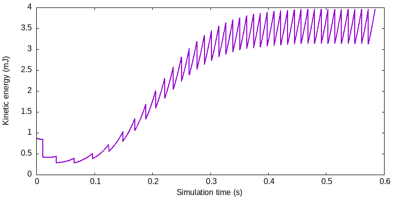
Notice that the first collision — one domino on one domino — loses half of the initial energy that was supplied from pushing. The subsequent acceleration is meagre as well, with the first domino struggling to push the second domino over its pivot point. But as more dominoes in the train start to fall together, the potential energy loss (and thus kinetic energy gain) during each acceleration cycle increases. Eventually, an equilibrium is reached where the kinetic energy gain in each cycle is equal to the kinetic energy loss in each collision².

The below graph shows this in terms of the angular velocity of the leading domino (N.B. here we are following the leading domino at any given time, so each saw tooth is actually a new domino):

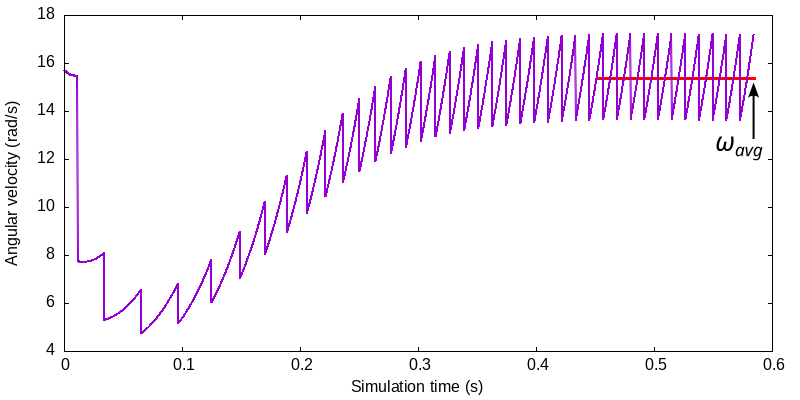
The red line shows the average angular velocity once equilibrium is reached, we will denote this by ω_avg. From this we can calculate the linear velocity v of the domino wave front, via:

(10) $\begin{align*} T &= \frac{\theta_c}{\omega_{avg}} \quad\text{(fall time)} \\ &= \frac{\sin^{-1}(\frac{\lambda-d}{L})}{\omega_{avg}} \\ v = \frac{\lambda}{T} &= \left(\frac{\lambda}{\sin^{-1}(\frac{\lambda-d}{L})}\right)\omega_{avg} \\ & \approx \left(\frac{\lambda}{\lambda-d}\right) L \omega_{avg} \quad\text{if }\tfrac{\lambda-d}{L} \text{ small} \end{align*}$

The approximation here ignores the curvature of each domino’s fall (Lω_avg is the average tangential velocity, rather than the average horizontal velocity), thus slightly overestimating the linear velocity. The leading factor $\tfrac{\lambda}{\lambda-d}$ can be seen as correcting for the travel of the wave front through the physical dominoes. That is, we assume that as soon as a domino is hit on one side, the far side starts moving instantaneously. So each time the falling wave front travels by λ-d, the domino thickness d is obtained for free. This is also very close to true in practice: the shock wave travels at the speed of sound (approximately 2250 m/s in ABS plastic) which is much much faster than the velocity during falling (typically <1 m/s).

While we can determine ω_avg from simulation, ideally we would like to find a closed form expression for it, so that we can understand its dependence on parameters such as domino spacing and geometry. Unfortunately this is elusive; it requires integration of the acceleration, which is a very complex function (see equation (5)). But with some simple arguments about energy, we can obtain expressions for ω₊ and ω_–, at least for the frictionless case. Then we can interpolate an approximation for ω_avg.

Assume that the domino train is well developed, i.e. many dominoes have already toppled and the equilibrium state is reached. Then each time the train moves forward by one domino, it releases one domino’s worth of potential energy (that is, potential energy equivalent to one domino falling from the upright position to the most toppled position). We can see this by observing the change as the line moves forward by one domino — the configuration is the same except for one upright domino being replaced with one toppled domino:

We equate this decrease in potential energy to the increase in kinetic energy during the acceleration phase:

$\begin{equation*} mg \Delta h = I {\omega_{+}}^2 K(0) - I {\omega_{-}}^2 K(\theta_c) \end{equation*}$

Where Δh is the change in center-of-mass height between upright and toppled positions, K(θ₀) is the function that relates the kinetic energy of the whole system to that of the leading domino (as defined in equation (4)), and θ_c is the angle at collision. Now due to the geometry at collision, K(θ_c) = K(0)-1, so we can also write:

$\begin{equation*} mg \Delta h = I {\omega_{+}}^2 K(0) - I {\omega_{-}}^2 (K(0)-1) \end{equation*}$

At the collision the velocity changes from ω₊ back to ω_–. We can apply the collision law (equation (9)) with ω_i = ω₊ and ω_f = ω_–. Solving these two equations simultaneously gives us closed form expressions for ω₊ and ω_–:

$\begin{align*} \omega_{+} &= \sqrt{\left(\frac{K}{K-1}\right) \frac{2mg\Delta h}{I}}\\ \omega_{-} &= \sqrt{\left(\frac{K-1}{K}\right) \frac{2mg\Delta h}{I}}\\ &\quad\text{ where } K = K(0) \end{align*}$

We can also substitute in $I = \frac{1}{3}m(L^2+d^2)$ to eliminate m, leaving dependence on geometry and g only:

$\begin{align*} \omega_{+} &= \sqrt{\left(\frac{K}{K-1}\right) \frac{6g\Delta h}{L^2 + d^2}}\\ \omega_{-} &= \sqrt{\left(\frac{K}{K-1}\right) \frac{6g\Delta h}{L^2 + d^2}}\\ &\quad\text{ where } K = K(0) \end{align*}$

These expressions are exact for the case with no domino-domino friction, and match simulation. Now to estimate ω_avg, it would be very tempting to take the geometric mean: while this has no clear physical significance, it would eliminate the part of the expression involving K. The alternative is to take the arithmetic mean, which is equivalent to assuming constant acceleration during the acceleration phase. The following table evaluates the accuracy of these estimates, considering standard-sized dominoes at three different spacings:

Domino pitch λ	ω_–	ω₊	ω_avg (true)	ω_avg ≈ √ω₊ω_–	ω_avg ≈ ½(ω₊+ω_–)
1.6cm	13.63	17.25	15.38	15.33 (-0.3%)	15.43 (+0.4%)
2.4cm	14.83	21.74	18.16	17.95 (-1.1%)	18.28 (+0.7%)
3.2cm	17.80	24.80	19.54	19.15 (-2.0%)	19.80 (+1.3%)

While this table represents a very limited set of parameter values, it seems that the geometric mean underestimates the true velocity while the arithmetic mean overestimates the true velocity. Let us stick with the geometric mean here since it allows us to eliminate K, and the underestimate here partially compensates for the overestimate in equation (10). Thus we take:

(11) $\begin{equation*} \omega_{avg} \approx \sqrt{\frac{6g\Delta h}{L^2 + d^2}}\\ \end{equation*}$

Δh can be expressed as:

(12) $\begin{align*} \Delta h &= \frac{L}{2} - \left(\frac{L}{2}\cos(\theta_f) + \frac{d}{2}\sin(\theta_f)\right) \\ & \qquad\text{ where }\theta_f = \cos^{-1}\left(\frac{d}{\lambda}\right) \text{ (final angle)} \\ &= \frac{L}{2}\left(1-\frac{d}{\lambda}-\frac{d}{L}\sqrt{1-\left(\frac{d}{\lambda}\right)^2}\right) \end{align*}$

Terminal velocity – finale

Combining equations (10), (11) and (12), we finally have:

(13) $\begin{align*} v &\approx \left(\frac{\lambda}{\lambda-d}\right) L \sqrt{\frac{3gL\left(1-\frac{d}{\lambda}-\frac{d}{L}\sqrt{1-\left(\frac{d}{\lambda}\right)^2}\right)}{L^2 + d^2}}\\ &= \sqrt{3gL} \sqrt{\frac{1-\frac{d}{\lambda}-\frac{d}{L}\sqrt{1-\left(\frac{d}{\lambda}\right)^2}}{\left(1-\frac{d}{\lambda}\right)^2\left(1+\left(\frac{d}{L}\right)^2\right)}} \end{align*}$

Now we have the approximate terminal velocity expressed in terms of a characteristic velocity $\sqrt{3gL}$ , and a velocity correction factor based on $\tfrac{d}{\lambda}$ and $\tfrac{d}{L}$ . For thin enough dominoes ( $d \rightarrow 0$ ), the correction factor approaches 1 and $v \rightarrow \sqrt{3gL}$ . However, very thin dominoes are not practical in the real world: firstly, they become increasingly difficult to stand up, and secondly, if the dominoes are very light then air drag and air turbulence come into play.

Even aside from this practicality, $\frac{d}{L}$ and $\frac{d}{\lambda}$ cannot take arbitrary values. Depending on the value of $\frac{d}{L}$ , there is a maximum $\frac{d}{\lambda}$ (a minimum spacing) for the domino line to successfully topple. Writing van Leeuwen’s equation (79) in terms of our symbols produces:

$\begin{equation*} \frac{d}{\lambda} < \frac{1-\left(\frac{d}{L}\right)^2}{1+\left(\frac{d}{L}\right)^2} \end{equation*}$

While this expression is elegant, unfortunately it is not sufficient: we find that, even in simulation, the domino line fails to propagate at a lower value. This could be a topic for further theoretical work. In any case, once we combine such a minimum spacing constraint with the requirement for the dominoes to actually hit each other (and ideally to stack), this constrains the valid ranges for the parameters.

The following plot shows the velocity correction factor from equation (13) for various valid values of $\frac{d}{L}$ and $\frac{d}{\lambda}$ , where the valid ranges were determined from simulation. Notice that the higher $\frac{d}{L}$ is, the smaller the valid range of $\frac{d}{\lambda}$ :

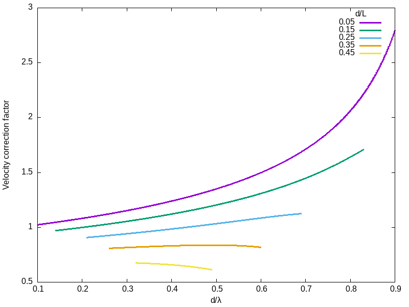
It is apparent that the velocity correction factor decreases with $\frac{d}{L}$ , that is with thicker dominoes. It generally increases with $\frac{d}{\lambda}$ , that is with decreasing spacing, except for the cases with very high $\frac{d}{L}$ . The increase with $\frac{d}{\lambda}$ is attributable to the actual dominoes spanning a greater proportion of the distance; if only velocity during falling were considered, all lines would be monotonically decreasing.

The following plot compares my equation to the power law model of Cantor & Wojtacki (2022), and simulation data, for standard commercial toppling dominoes with $\frac{d}{L}$ = 0.15625:

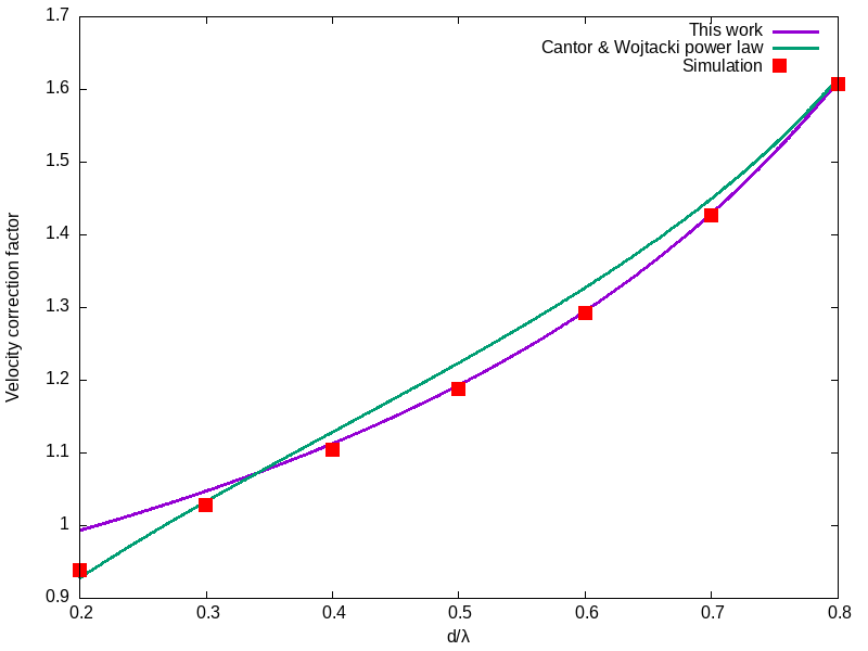
My approximation (purple line) fits well but deviates for small $\frac{d}{\lambda}$ (large spacing). This is attributable to the velocity approximation taken in equation (10); it is likely that a better approximation is possible, the challenge is to find one that simplifies rather than complicates the equations. Meanwhile the published power law approximation fits well at the extremities but not as closely in the middle.

Note again that the analysis in this section ignores friction between dominoes. Friction between dominoes does have a significant effect on the terminal velocity, and this is why we have not tried to correlate the results here with experimental data, only with simulation models with friction co-efficient μ set to zero. A theoretical approximation for the friction correction is left to future work. Cantor & Wojtacki provide an empirical velocity correction factor of (1+μ)^-0.4 based on their simulation studies.

Comparison between simulation and experiment

To validate the sanity of the simulation model, I also performed a few real world experiments. I used a set of H5 Domino Creations dominoes, which have standard toppling domino dimensions of 48mm(L) x 24mm(w) x 7.5mm(d). The domino-domino coefficient of dynamic friction was estimated to be approximately 0.25 ± 0.05³. In each experiment I built a line of 100 dominoes with known spacing using a template, and recorded the sound of them toppling. The “best fit” domino toppling frequency was determined via acoustic analysis (autocorrelation).

The results were compared with my simulation program, and a more sophisticated physics simulation using the LMGC90 program from Université de Montpellier. (All of the code used is in my github repository.)

The data is shown in the following table. Each cell shows toppling frequency in dominoes per second; if desired this can be converted to velocity by multiplying by domino pitch.

Domino pitch λ	Experiment	Simulation (mine)	Simulation (LMGC90)
1.6cm	64.4	59.7	59.1
2.4cm	42.3	37.2	36.9
3.2cm	28.1	26.2	26.1

My simulation model shows good fit to the LMGC90 simulation. However, both models appear to slightly underestimate the real world velocity. This is surprising, since normally one would expect theoretical simulations to overestimate the velocity, with more losses in the real world.

Let us revisit the model assumptions:

We assumed that there is sufficient friction with the floor that the dominoes do not slide. Slow motion video shows that a very small amount of sliding does occur on my floor. However, one would expect that sliding would dissipate energy and reduce the velocity, and this is confirmed in LMGC90 simulation when varying the floor friction coefficient. In any case, the LMGC90 simulation does not require making this assumption, and similar results are obtained.
We assumed that dominoes do not rotate in any axis other than the one corresponding to forward toppling. In practice, the dominoes are never placed perfectly parallel and some rotation is observed around the long axis of the dominoes. Again this causes slipping on the floor and would be expected to dissipate energy and reduce velocity.
We assume that each falling domino ends up leaning on the next one a “short time” after collision. In my slow motion video (around time 1:05 and 4:30), the time period seems to be short, however Destin Sandlin’s slow motion video (around time 4:50) shows lack of contact for a longer time. If the time period is not negligible, not only is the collision law affected, but there is no friction between these front two dominoes during the time that they are not in contact. It is possible that this could increase the velocity compared to simulation.

There are two other implicit assumptions in the simulations:

We implicitly assume perfect placement of dominoes, which is not possible in the real world. The effect of placement deviations requires further study.
We implicitly assume Amonton’s/Coulomb’s laws of friction hold. Even if the coefficient of friction could be measured precisely, these linear friction relationships are inherently approximations.

Conclusion

In this article, I showed how to derive the equations of motion for a toppling domino line, under certain assumptions. I used these equations of motion to build a simulation program, and the results of the simulations show good agreement with 3D physics simulation in LMGC90. I also applied energy conservation arguments to derive approximate expressions for terminal velocity, at least for an ideal case with no domino-domino friction. Surprisingly, my real world experiments show slightly higher velocities than simulations, which may be to do with the collision dynamics. As so often occurs in physics, something that seems quite simple turned out to be quite a rabbit hole.

Footnotes

There is one thing I have brushed under the carpet here, which is the evaluation of K’. With some working we can obtain:

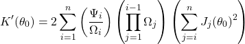
which is not exactly nice, but does the job for numerical simulation. If anyone finds a simpler expression, let me know. ↩︎
Mathematically speaking, equilibrium is never perfectly reached, it is merely approached. In fact the potential energy released per cycle continues to increase, ever more infinitesmally with each extra domino. But practically speaking this is a moot point. ↩︎
The standard method of measuring the coefficient of dynamic friction is to slide an object of one material down a ramp of the other material, and to determine the ramp angle at which the object slides at constant velocity. Doing this rigorously with dominoes proved difficult since my “ramp” had slight discontinuities where I had adhered the dominoes together, however based on many attempts I bounded the coefficient to this range. ↩︎