Splines in Onshape, part 1

Introduction

First can I say how much I love Onshape. I have no association with the company other than being a user, so you can trust that this is real, genuine puppy love. Onshape provides much of the functionality of parametric CAD systems such as SolidWorks in your browser, which at first sight seems like magic. Since I’m a Linux user and the native CAD landscape on Linux is quite limited, being able to do CAD in a browser works brilliantly for me. Even better, it’s free for non-commercial use.

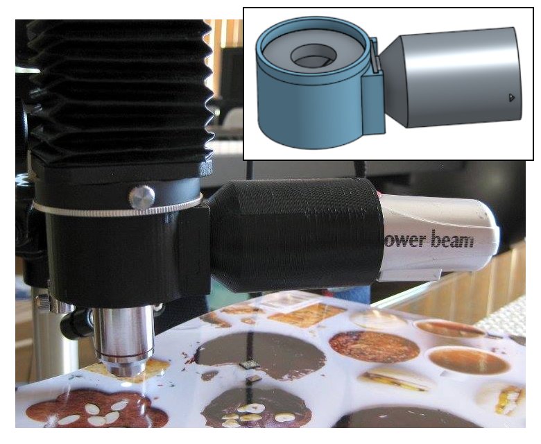
My first little project in Onshape, several moons ago, was a vertical illuminator for my home-brew microscope. The problem I had was that when using high magnifications — which require the lens very close — I couldn’t get enough light in under the lens to illuminate opaque samples. A vertical illuminator is the solution to this problem, sending light down through the lens via a beamsplitter. I designed the physical parts in Onshape, exported to STL format and uploaded to Hubs (previously 3DHubs); a local maker printed the parts and within a few days I had it back and working.

Scripting in Onshape

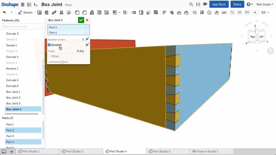
Onshape has a scripting language called FeatureScript. FeatureScript allows extending the Onshape interface with domain-specific tools (features as they’re known in Onshape). For example, if you are doing furniture design in Onshape, you can write features that produce panels and joints and then do high-level design in the user interface, rather than having to work with low-level primitives such as lines and boxes. Clearly this can be a huge boon to productivity. Here is a screenshot from one of the Onshape demonstration videos showing a custom box joint feature that, once created, can be used just like built-in features:

As a programmer and perfectionist I like the idea of writing code to simplify the CAD process rather than spending hours placing parts in a GUI. Prior to Onshape I’ve used OpenSCAD a few times. But for complex designs it gets difficult to mentally keep track of what’s where without having a live preview, and OpenSCAD rendering can get very slow once you start chamfering, filleting and making things pretty. This is where Onshape and FeatureScript shine.

Recently I’ve been doing a bit of jewellery design in Onshape, and this involves a lot of curves and curved surfaces. While I can approximately create the curves I want in the GUI, I wanted to do it programmatically in FeatureScript. Unfortunately a number of the functions that I needed to use were minimally documented so I had to do a lot of trial and error in the process. This article is an attempt to explain some of the missing links for those following in my footsteps.

Onshape is still being developed at a breakneck pace, and since I started writing this article there are now a number of new features related to curves including the option to directly create splines in 3D. I’ll start, though, from the ‘traditional’ way of creating curves in Onshape — by creating them in a 2D sketch and then lofting/extruding/etc. — and I’ll briefly mention 3D curves later in the piece.

Basics of splines

There’s a lot of mathematical jargon around splines and polynomials, so I’ll try to use both the technically correct terms and plain English where possible.

A spline is a piecewise polynomial. The curve is made up of one or more pieces, where each piece is a polynomial. The polynomials are normally chosen such that they “match up” at the transitions and you end up with something that looks like a single continuous curve. There can be various definitions of “matching up”, however to produce a visually smooth curve, at least the function values and the first derivative need to match (C1 continuity), and usually the second derivative is also chosen to match (C2 continuity).

In the case of Onshape splines used in sketches, the pieces are normally cubic polynomials — polynomials of maximum degree 3 — in two dimensions x and y. However, I should be clearer what I mean by that, as there could be at least three different things that could be meant by cubic polynomials in two dimensions:

Explicit form: y=f(x):
y = ax³ + bx² + cx + d
(defined uniquely by 4 free constants: a,b,c,d)

Parametric form: x=f(t), y=g(t) for some parameter t:
x = at³ + bt² + ct + d
y = et³ + ft² + gt + h
(defined uniquely by 8 free constants: a,b,c,d,e,f,g,h)

Implicit form: f(x,y)=0:
ax³ + bx²y + cxy² + dy³ + ex² + fxy + gy² + hx + ky + l = 0
(defined uniquely by 10 free constants: a,b,c,d,e,f,g,h,k,l)

The explicit form can produce, say, a parabola y=x², but can’t produce a parabola rotated by 90 degrees. Therefore it makes little sense for software such as Onshape which must be able to produce curves in any orientation.

The implicit form is the most powerful, in that it can express curves that can’t be expressed in the other two forms, but it is difficult to evaluate the set of points that are part of the curve.

Therefore, as might be expected, Onshape curves are of the parametric type: a curve in two dimensions is produced parametrically by evaluating functions x(t) and y(t) for t from 0 to 1. The functions x(t) and y(t) are splines: there may, for example, be one polynomial piece from t=0 to t=0.5 and one from t=0.5 to t=1. Some of the FeatureScript functions related to curves, such as evEdgeTangentLine() and evEdgeCurvature(), take this parameter t as an argument.

Drawing 2D splines – single polynomial piece

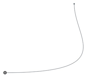
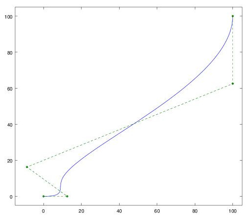
Splines can be created programmatically in an Onshape sketch using the skFitSpline() function. First let’s start with a curve with only one polynomial piece between two points (0,0) and (100,100). In FeatureScript we can write:

skFitSpline(sketch, "spline1", {
        "points" : [
            vector(0,0) * meter,
            vector(100,100) * meter
        ],
        "startDerivative" : vector(150,0) * meter,
        "endDerivative" : vector(0,150) * meter
});

Here is the result:

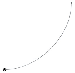
Note that I’ve specified a startDerivative and endDerivative that specify the starting and ending direction; if I had only specified a start and end point then the result would have just been a straight line.

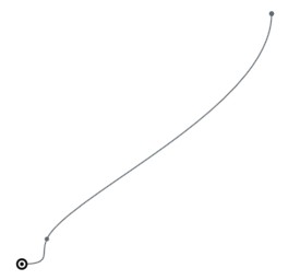
When I was first experimenting with this, my first question was: why do the start and end derivatives have length units (in this case, 150 meters)? With a bit of experimentation it’s clear that these these vectors should be scaled together with the curve, i.e. if we scale the curve up by a factor of two we should also double the startDerivative and endDerivative. Also, a larger magnitude makes the curve launch with more momentum in the given direction; for example, here is the curve with startDerivative increased to (500 meters,0):

But what does the magnitude of these vectors actually mean?

It all becomes clearer, however, when you consider the curves in parametric form as described in the previous section: x=f(t) and y=f(t). It turns out that the given derivative vectors are the derivatives of (x(t), y(t)) with respect to the parameter t (i.e. (dx/dt, dy/dt)) at t=0 and t=1. If this is too abstract to visualize, there is also a simple mapping to Bézier control points that I’ll explain below.

It turns out that the start point and end point, and the two derivative vectors – four (x,y) pairs in total – uniquely define the eight parameters of the parametric cubic polynomial. Thus, any parametric cubic polynomial can be specified in this way.

If you don’t specify the derivative at the start point or end point, the second derivative at that point is set to zero, which is sufficient to provide the missing constraint on the polynomial.

Drawing Bézier curves

If you are familiar with Bézier curves the above discussion will sound familiar. A Bézier curve is defined by four control points (call them P₁, P₂, P₃, P₄). The curve launches from P₁ in the direction of P₂, and then approaches P₄ from the direction of P₃. If P₂ is further away from P₁, then the curve launches with more momentum in the given direction.

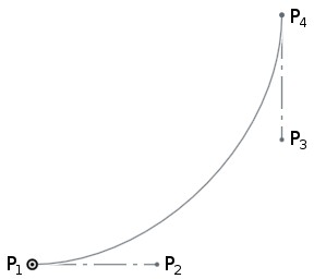
It turns out that these formulations are equivalent with a tiny amount of maths, and if you have the Bézier control points, you can calculate the required startDerivative and endDerivative as:

(1)  

where Δt will be 1 for the simple case that t varies from 0 to 1 across the curve segment, and the 3 arises from the degree of the polynomial (because d/dt(t³) = 3t²). Thus, for a single-piece spline, the startDerivative and endDerivative will be three times the distance to the corresponding Bézier control point.

Of course you can also calculate the Bézier control points from the startDerivative and endDerivative by rearranging these equations for P₁ and P₂:

(2)  

Evaluating splines in Onshape

You can evaluate the spline at any point using the evEdgeTangentLine() function in FeatureScript, providing the parameter value t (from 0 to 1). The Line object that is returned has an origin that provides the evaluated point and has a direction that is tangent to the spline.

var curve = qCreatedBy(id + "sketch", EntityType.EDGE);
var tangent = evEdgeTangentLine(context, {
        "edge": curve,
        "parameter": 0.5,
        "arcLengthParameterization": false
});
println(tangent.origin);
println(tangent.direction);

Debug pane output:
(68.75 meter, 31.25 meter, 0 meter)
(0.7071067811865475, 0.7071067811865475, 0)

This can be useful for performing further geometry calculations after drawing a spline. For completeness I’ll note that there is also a evEdgeTangentLines() function — which is identical but allows evaluating the curve at multiple points in one call — and an evEdgeCurvature() function — which returns not only a tangent but also normal and binormal vectors.

Drawing 2D splines – multiple polynomial pieces

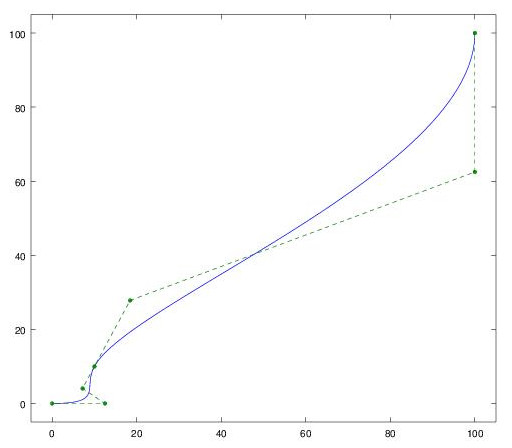
Now let’s add another point to the spline:

skFitSpline(sketch, "spline1", {
        "points" : [
            vector(0,0) * meter,
            vector(10,10) * meter,
            vector(100,100) * meter
        ],
        "startDerivative" : vector(150,0) * meter,
        "endDerivative" : vector(0,150) * meter
});

Here is the result:

Now there are two polynomial pieces, one that goes from (0,0) at t=0 to (10,10) at t=0.25, and one that goes from (10,10) at t=0.25 to (100,100) at t=1. The breakpoint between the two – called a knot – is at t=0.25.

Why is the knot at t=0.25? Well, this knot could actually be placed anywhere in ‘t space’, for instance t=0.1 or t=0.5, but as the second piece of the curve is much longer there is an argument for assigning more ‘t space’ to the second piece. Onshape uses the square root of the chord length between points as the metric; the lengths of the two chords here are 14.1m and 127.3m so the knot location is chosen as sqrt(14.1m)/(sqrt(14.1m)+sqrt(127.3m)) = 0.25.

The polynomial pieces are chosen such that both the first and second derivative are continuous through the middle point, which uniquely defines the two polynomials. The resulting curve ends up being the same as what would be produced by the following two skFitSpline calls:

skFitSpline(sketch, "spline1.piece1", {
        "points" : [
            vector(0,0) * meter,
            vector(10,10) * meter
        ],
        "startDerivative" : vector(37.5,0) * meter,
        "endDerivative" : vector(8.4375,17.8125) * meter
});
skFitSpline(sketch, "spline1.piece2", {
        "points" : [
            vector(10,10) * meter,
            vector(100,100) * meter
        ],
        "startDerivative" : vector(25.312,53.438) * meter,
        "endDerivative" : vector(0,112.5) * meter
});

… where I’ve calculated the required piece1 endDerivative and piece2 startDerivative so that both first and second derivatives match at the joining point (10,10). Note that all of the derivatives end up scaled when splitting the curve, as they are derivatives with respect to t and t is no longer the same variable (now each piece has t from 0 to 1).

As a corollary, if you only care about first derivative continuity and not second derivative continuity, then you can actually get a larger variety of curves by drawing the two parts individually: then you can choose any value for the piece1 endDerivative and piece2 startDerivative as long as the direction matches.

B-splines

Actually Onshape represents all of these splines in terms of B-splines rather than as an array of polynomial co-efficients a,b,c,d,e,f,g,h for each piece. Contrary to popular belief, there is nothing voodoo about B-splines, they are just a tool for expressing splines in a more convenient form.

The basic idea is that we can separate a spline function into a set of control points c, which define an approximate path for the spline, and a set of functions b(t), which give the weighting of each control point at a parameter value t along the curve. The spline may not pass through all or even any of the control points c, but moving the control points allows you to control the path of the curve.

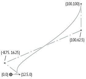
For example, the control points for the spline that we generated in the previous section are are depicted below (I’ll explain how these are determined from the skFitSpline() parameters in a moment):

If we think of c as a column vector of control points and b(t) as a row vector, then at any point we can evaluate the spline function as:

(3)  

b(t), which weights the control points, is chosen such that it has a number of nice properties. The sum of components in b(t) should always be 1 for any t, which is required for scale-invariance (i.e. if you scale up the control polygon c, the spline should scale with it). Also, b(t) should be smooth everywhere (i.e. continuous first and/or second derivatives), such that s(t) is smooth everywhere.

A suitable function b(t) can be generated using what’s called the Cox-de Boor recursion formula. The only input to this algorithm is an ordered list of t values called knots – these are transition points between a set of underlying polynomials used to construct b(t).

To make it easy to experiment with B-splines, I wrote a simple Octave/MATLAB function that generates b(t) for a given polynomial degree and a given set of knots. The code is here: bsplinebasis.m. For example, for the previous curve with a knot at 0.25, we can evaluate:

octave:1> degree=3;
octave:2> knots=[0,0,0,0,0.25,1,1,1,1];
octave:3> bsplinebasis(degree, knots, 0.5)
ans =

   0.00000   0.16667   0.44444   0.35185   0.03704

In other words, at t=0.5, the five control points of the spline are weighted according to this vector. Notice that here (and in fact anywhere beyond the first knot at t=0.25) the first control point has no effect; this is a B-spline property called local support.

I’ve failed to explain something. It makes sense that the knot locations are at t=0,0.25,1, which corresponds to the pieces of the spline, but notice that I’ve repeated the t=0 and t=1 knots four times on line 2. This is called knot multiplicity. In order for the spline to be “clamped” to the first and last control points, these knots must be repeated at least n+1 times (where n is the degree of the polynomial). A picture that illustrates this can be found on this website.

We can now draw the spline in Octave and confirm that it looks the same as in Onshape, and indeed it does:

octave:4> t=[0:0.01:1];
octave:5> cpts=[0+0i; 12.5+0i; -8.75+16.25i; 100+62.5i; 100+100i];
octave:6> plot(bsplinebasis(degree,knots,t)*cpts,'-',cpts,'--.')

In the above code I’ve expressed the control points as complex numbers x+iy as a convenience. I could also have done, equivalently:

octave:7> xcpts=[0; 12.5; -8.75; 100; 100];
octave:8> ycpts=[0; 0; 16.25; 62.5; 100];
octave:9> plot(bsplinebasis(degree,knots,t)*cxpts,
                   bsplinebasis(degree,knots,t)*cypts)

Note that the control points are not the same as the points you specify to skFitSpline(). In this example, the specified points to skFitSpline() were (0,0), (10,10), (100,100) with startDerivative of (150,0) and endDerivative of (0,150), while the corresponding spline control points are (0,0), (12.5,0), (-8.75,16.25), (100,62.5), (100,100). How did I arrive at these control points? The first and last fit points become the first and last control points. The second and second-last control points can calculated from the startDerivative and endDerivative using equation set 1. The other control points are derived from the remaining fit points with linear algebra, using equation 3.

You can create a a spline with a given set of control points and knots directly using skSplineSegment() as follows:

// Not recommended, not a public API
skSplineSegment(sketch, "spline2", {});
var guess = {"spline2": [
               0, // isClosed
               0, // isRational
               3, // degree
               5, // numControlPoints
               0,0,12.5,0,-8.75,16.25,100,62.5,100,100, // pts
               0,0,0,0,0.25,1,1,1,1, // knots
               0, // lowParameter
               1  // highParameter
               ]};
  skSetInitialGuess(sketch, guess);
  skSolve(sketch);

Note however that however this is not a public API and subject to change, so it’s better to use skFitSpline() where possible. If you want to define a spline using control points, you can easily convert it to skFitSpline() form by evaluating it at all of its knots, and calculating the startDerivative and endDerivative using equation set 2.

(For completeness, there are actually at least four internal functions that produce splines: skSpline(), skSplineSegment(), skInterpolatedSpline() and skInterpolatedSplineSegment(). The ‘Interpolated’ versions take a set of points the curve passes through plus the start and end derivatives, while the non-interpolated versions take control points. The ‘Segment’ functions produce an open spline with endpoints, whereas the non-segment functions can be used for closed splines without endpoints. skFitSpline() is a more user-friendly version of skInterpolatedSplineSegment().)

Why B-splines?

It can be seen that the B-spline form of a spline has a number of advantages over specifying polynomial co-efficients for each polynomial piece. Firstly the control points have a more intuitive geometric interpretation than the polynomial co-efficients. Secondly, if b(t) is chosen to have second-derivative continuity, then s(t) automatically has second-derivative continuity without needing to fit a set of co-efficients that satisfy this criterion. However there is nothing magic about B-splines: you can calculate the polynomial co-efficients from the B-spline control points, and vice versa, so they are just different representations of the same curves.

Note also that for a single-piece spline with a simple knot vector like [0,0,0,0,1,1,1,1], b(t) is exactly equivalent to the weighting that defines a Bézier curve, and the resulting spline is the same as the Bézier curve with the same control points. More complicated splines can be decomposed into multiple such Bézier pieces. So again there is nothing more or less powerful about these splines versus a set of Bézier curves joined together; however the B-spline representation requires less control points for the default case that second-derivative continuity is desired.

In fact I’ll admit to a little sleight-of-hand when preparing this article, where I’ve used the properties of B-splines to make my life easier. In one of the sections above, I split the curve created by skFitSpline() into its two equivalent pieces. The first time I did this, I did it from first principles — writing down the curves in polynomial form and setting the second derivatives equal at the joining point — and it took me a few pages of working. When I needed to redo it for the example spline in this article, though, I used an easier method which is to split the B-spline using a knot insertion algorithm. This is a method for inserting extra knots (and calculating updated control points) while preserving the same curve. By inserting two extra knots at t=0.25, the control polygon can be made to pass through the point (10,10) and we now have two explicit Bézier pieces. Here is the process I used in Octave:

octave:10> cpts,knots
cpts =

     0.00000 +   0.00000i
    12.50000 +   0.00000i
    -8.75000 +  16.25000i
   100.00000 +  62.50000i
   100.00000 + 100.00000i

knots =

   0.00000   0.00000   0.00000   0.00000   0.25000   1.00000
   1.00000   1.00000   1.00000

octave:11> [cpts,knots]=bsplineinsert(degree,cpts,knots,0.25)
cpts =

     0.00000 +   0.00000i
    12.50000 +   0.00000i
     7.18750 +   4.06250i
    18.43750 +  27.81250i
   100.00000 +  62.50000i
   100.00000 + 100.00000i

knots =

   0.00000   0.00000   0.00000   0.00000   0.25000   0.25000
   1.00000   1.00000   1.00000   1.00000

octave:12> [cpts,knots]=bsplineinsert(degree,cpts,knots,0.25)
cpts =

     0.00000 +   0.00000i
    12.50000 +   0.00000i
     7.18750 +   4.06250i
    10.00000 +  10.00000i
    18.43750 +  27.81250i
   100.00000 +  62.50000i
   100.00000 + 100.00000i

knots =

   0.00000   0.00000   0.00000   0.00000   0.25000   0.25000
   0.25000   1.00000   1.00000   1.00000   1.00000

octave:13> plot(bsplineeval(degree,cpts,knots,t),'-',cpts,'--.')

Now control points 1 to 4 and control points 4 to 7 define two Bézier curves, and we can compute the required startDerivative and endDerivative values:

octave:13> startDerivative1 = (cpts(2)-cpts(1))*3
startDerivative1 =  37.500
octave:14> endDerivative1 = (cpts(4)-cpts(3))*3
endDerivative1 =   8.4375 + 17.8125i
octave:15> startDerivative2 = (cpts(5)-cpts(4))*3
startDerivative2 =  25.312 + 53.438i
octave:16> endDerivative2 = (cpts(7)-cpts(6))*3
endDerivative2 =    0.00000 + 112.50000i

I’ve uploaded the code for bsplineinsert.m to my GitHub along with some other B-spline utility functions.

Taking a break

Hopefully in this instalment you’ve learnt a few things about splines and how they can be represented in Onshape… I know I have. In part 2, I discuss offset splines, derivatives of splines, creating splines directly in 3D, and some other tidbits about Onshape internals.